QGIS 进阶

Post in 周三 12 一月 2022 |Tags GIS QGIS Python Learning Book

本文英文原版地址

地理信息系统流程自动化和高级可视化技术

英文原作者：Ujaval Gandhi

中文翻译：CycleUser

导论

本课程关注于地理信息系统工作留的自动化。本章你将学到更有生产力的技术，来创建美观的可视化，并解决复杂的空间分析问题。本课程尤其适合已经使用QGIS的人来提升进阶技能。

本文涉及的内容如下：

处理框架-算法、批处理和建模器
动画演示时间序列数据
从航拍图像创建立体透视图
高级表达式，实现快速数据编辑、模糊匹配等功能

进行练习之前，可以先了解一下关于QGIS的基础知识。

查看幻灯片提取码: 6npb

软件

本课程使用的软件是QGIS长期支持版本（LTR）3.16。

可以参考QGIS-LTR 安装指南。

获取数据包

本课程的样例要用到多种数据集。所有需要的图层、项目文件等等，都在下面的advanced_qgis.zip文件中。建议解压缩后将其放在Downloads文件夹下。

下载数据包提取码: 5r2l

处理框架（Processing Framework）

QGIS 2.0 开始引入了一个新概念，叫做处理框架（Processing Framework）。处理框架提供了在QGIS那运行原生或者第三方算法来处理数据的环境。这也是现在用于在QGSI那进行任何类型数据处理和分析的推荐方法，可以进行特征选择、属性修改和图层保存等等，当然这些也可以通过其他渠道来实现。不过使用处理框架会让这些工作更加有效率、更快速，还不容易出错。

处理框架包含下面这些不同的元素，一起配合工作。

处理工具箱 Processing Toolbox: 包含各种独立工具和算法，通过供应者和功能进行分类
批处理界面 Batch Processing Interface: 允许任何处理工具可以同时对多个图层执行
图形化建模器 Graphical Modeler: 允许用户定义工作流然后将多个处理步骤链接起来，使用拖拽机制（drag-and-drop mechanism）
历史管理器 History Manager: 记录存储算法进行的所有操作，允许用户重现过去的分析步骤
结果查看器 Results Viewer: 查看数据表和图表等算法产生的非空间输出结果

查看幻灯片提取码: nvbs

接下来就分章节来练习一下这些模块。（译者注：由于QGIS默认界面是英文的，后文中这几个模块的英文在文中就不再翻译了，直接用原文。）

处理工具箱（Processing Toolbox）

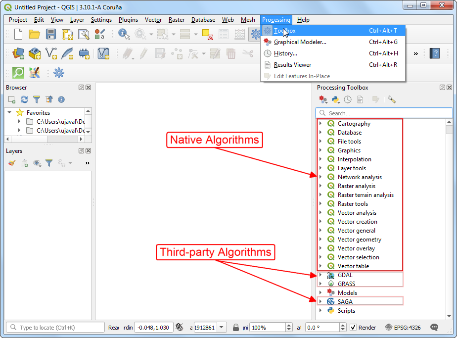
Processing Toolbox 可以在最顶层菜单Processing → Toolbox中找到。其中有几百个现成的算法。通过提供者Providers进行分类。由QGIS开发者创建的工具就在原生QGIS提供者（Native QGIS provider）分组中。处理框架（Processing Framework）提供了一种简单方式来集成其他软件和库，比如GDAL、GRASS和SAGA等等。QGIS的插件也可以通过在工具箱里面的处理算法增加新功能。

为何要使用处理算法（Processing Algorithms）

经过妥善测试和严格实现
主要用C++编写，运行速度比其他替代品更快
可以在后台运行长处理，不影响QGIS的前台使用
多线程算法可以充分利用多核心处理器，提高性能表现
健壮地处理无效几何体
可以查看运算过程并取消
可以在所有特征或所选特征上运行

查看默认设置

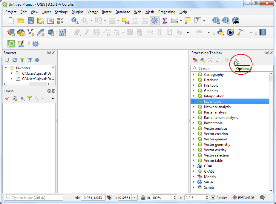
在设置中可以控制所见的处理工具提供者。处理选项菜单（Processing Options menu）也提供了框架设置的精细调整方式。

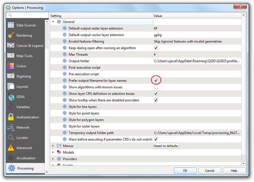
强烈推荐修改一下默认设置，启用选项Prefer output filename for layer names。这确保当你使用批处理的时候，得到的各个图层是唯一的。

练习: 找到州内的国家高速公路长度

该练习展示如何使用纯处理工作流解决多步骤的空间数据分析问题，以及QGIS中算法的丰富性，可以进行之前需要插件或者更复杂步骤的复杂操作。

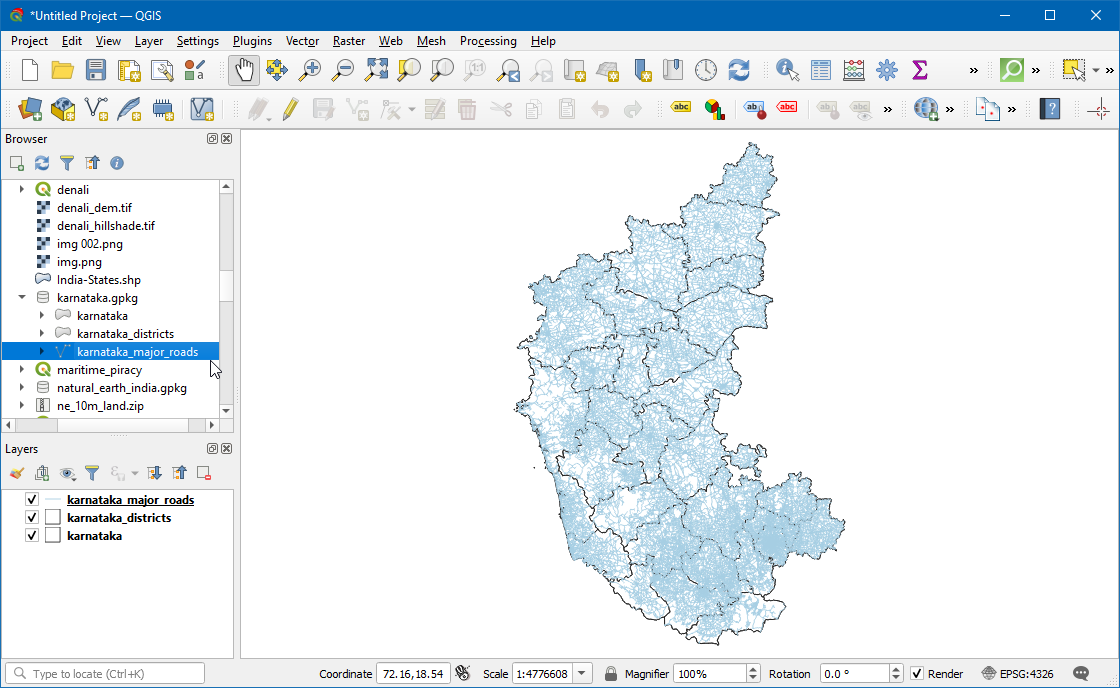
接下来从OpenStreetMap地图提取印度卡纳塔克（Karnataka）的道路信息。州的行政边界信息可以从DataMeet获得。

浏览文件夹定位到karnataka.gpkg，拖拽karnataka、karnataka_districts和karnataka_major_roads到QGIS地图画布中。

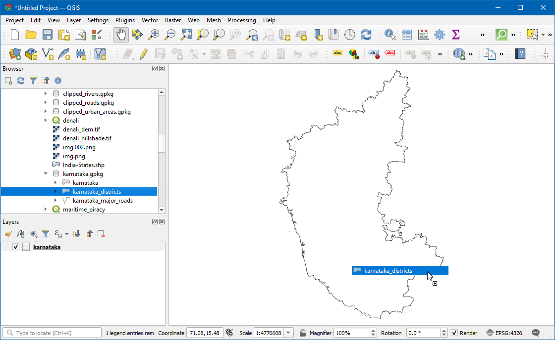
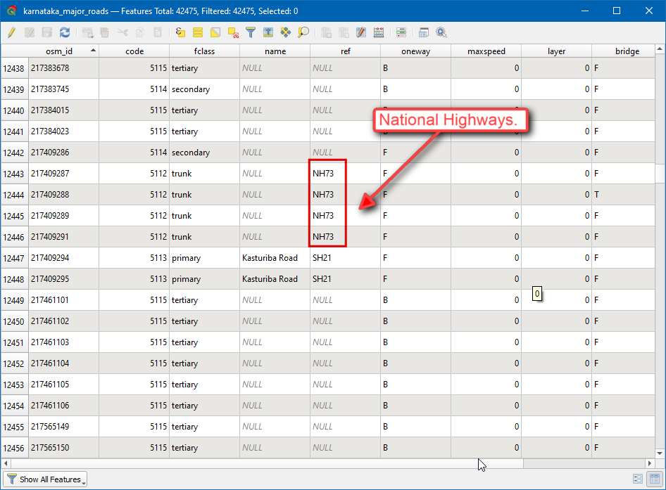
图层karnataka_major_roads包含了所有的主要道路，其中有国家高速公路、省级高速公路、主干道路等等。选择该图层，然后使用快捷键F6打开属性表格（attribute table）。

你会注意到ref这一列由关于道路的相关信息。由于本次练习中只需要国家高速公路，可以使用这列信息来只提取相关的道路段。

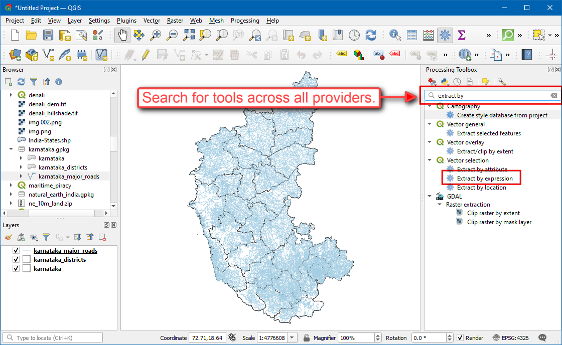
你可以使用通过表达式选择（Select by expression）工具，导出所选特征作为新图层，然后继续处理。但处理工具箱（Processing Toolbox）提供了一个更简单的无缝工作流，可以搜索算法Extract by expression。

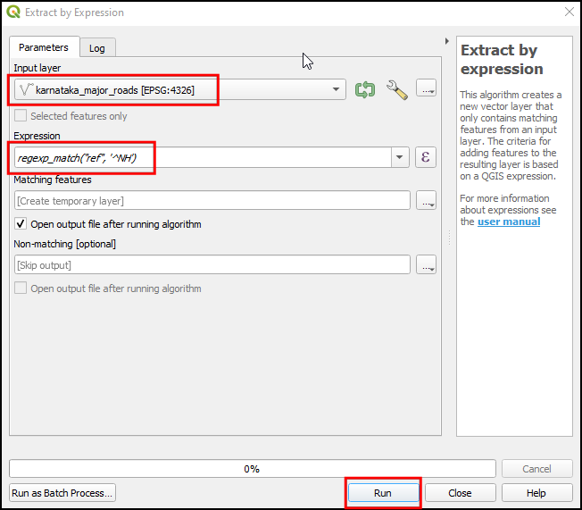
输入下面的表达式来提取特征，其中ref的开头字母为NH。

这里使用的其实就是正则表达式（Regular Expression，缩写为RegEx）来进行特定模式的匹配。正则表达式非常强大，可以用于很多复杂的数据筛选操作。基础细节可以参考这个链接。

regexp_match("ref", '^NH')

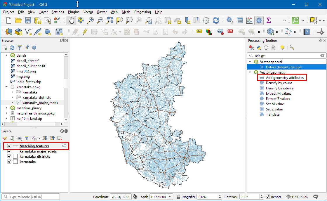
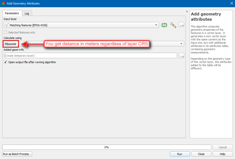
你会在图层面板（Layers Panel）得到一个名为Matching Features的新图层。接下来想要计算其中每个道路段的长度。可以使用内置算法Add geometry attributes。

源图层的地理坐标参考系（Geographic CRS）是EPSG:4326。但对此分析来说，要使用米或者千米来作为单位。算法提供了方便的选项来使用椭球体Elliposidal数学来计算距离，这对于地理坐标参考系的图层很适合。

添加了length值域的新图层就会被添加在图层面板中来。这个域的值的单位是米。然后转换成千米。这可以使用QGIS的域计算器Field Calculator 来增加一个新域（field）。这个方法绝对颗星，但还有一个更推荐的处理框架方法。搜索并打开Field Calculator 处理算法，然后输入下面的表达式。

"length"/1000

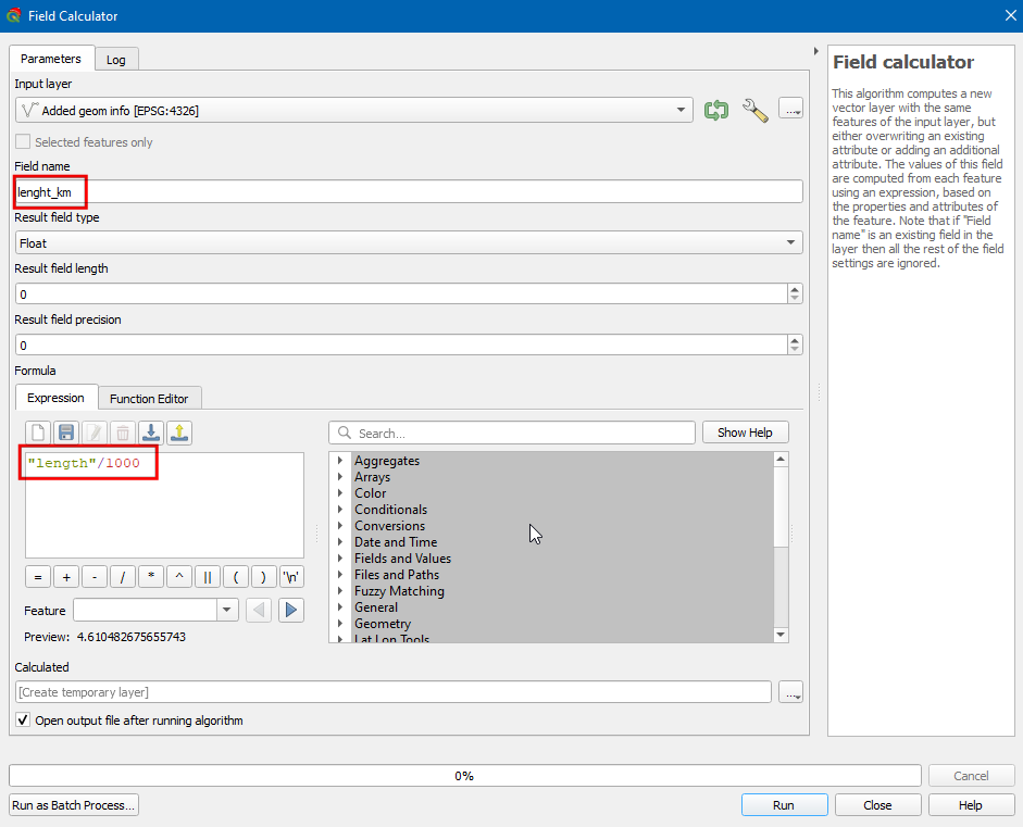
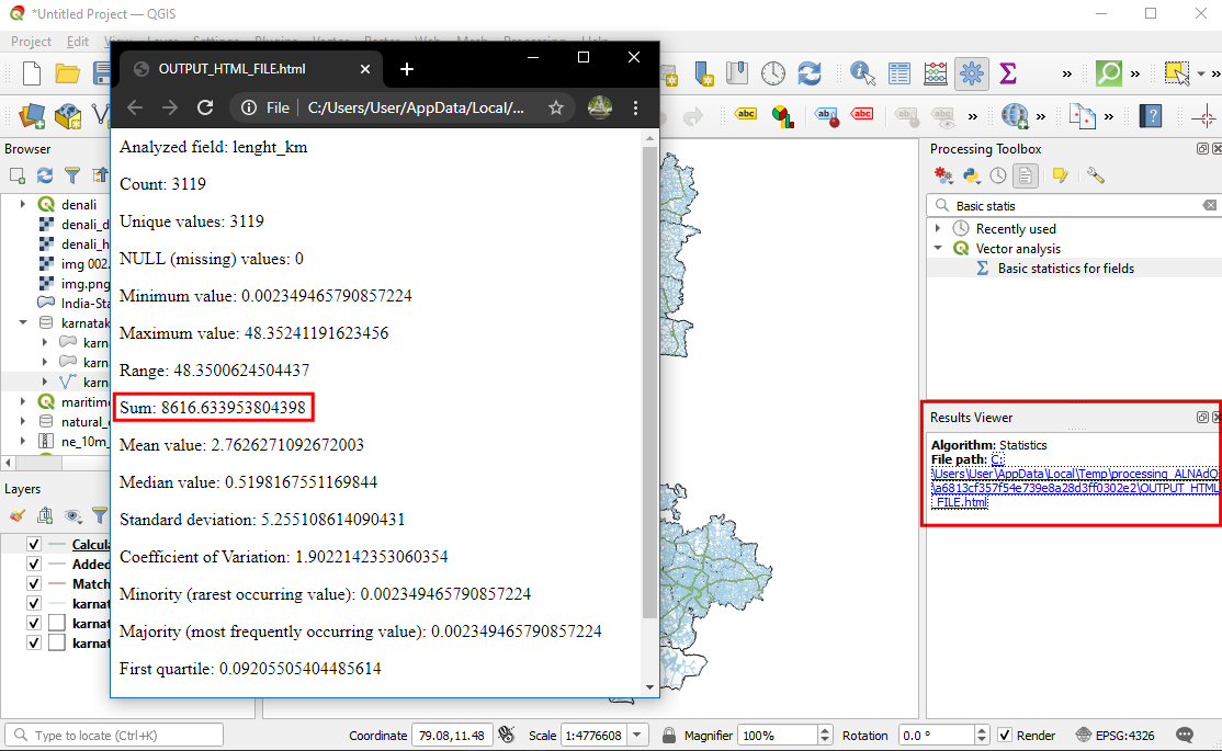
图层面板添加了带有域length_km的新图层。然后就是要解决问题了。只需要将新增图层中length_km的所有值加起来就可以了。使用Basic Statistics for Fields算法即可。

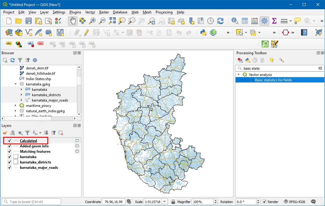
在Basic Statistics for Fields对话框中，选择Calculated作为输入层Input layer，选择length_km作为Field to calculate statistics on。点击Run运行。

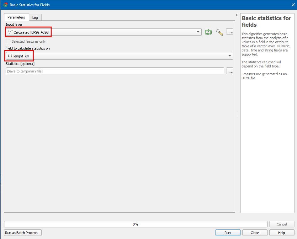
得到的结果是对列进行不同统计的数据表。由于结果不是图层，就要在Results Viewer中查看。图层面板中会包含一个HTML文件，包含的是统计值。Sum包含的就是该州内的所有国家高速路的长度。

你觉得结构怎么样？可能并不是很理想，因为OpenStreetMap数据库可能会有丢失的路径或者可能有分类错误。但应该和官方统计还是很接近的。

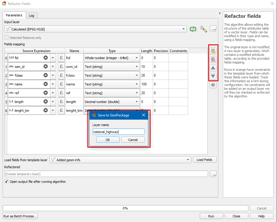
Calculated就是最终图层，也是一个临时的记忆层。将其保存到磁盘，以备后续使用。这个图层中有很多数据都是我们用不上的，所以可以删除掉一些列，然后字啊保存。经典方法是打开编辑模式然后在属性表格里面使用Delete Column按钮。如果你要重命名或者重新编码某个域，就需要一个插件。不过现在，我们已经可以使用Refactor Fields这样的处理算法来一次行进行加减、重命名和重新编码特定域。删除掉不需要的域，然后将结果存储为图层national_highways，保存在karnataka.gpkg中。

图层面板中新增了national_highways图层。这样就达到了本练习的目的，但还可以继续探索一点，如果可以将结果拆解成一个更小的行政单元。然后再计算一下每个小的行政单元内的国家高速公路长度。

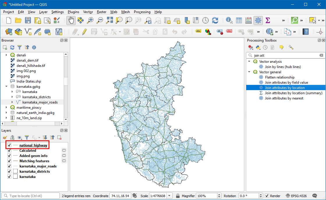
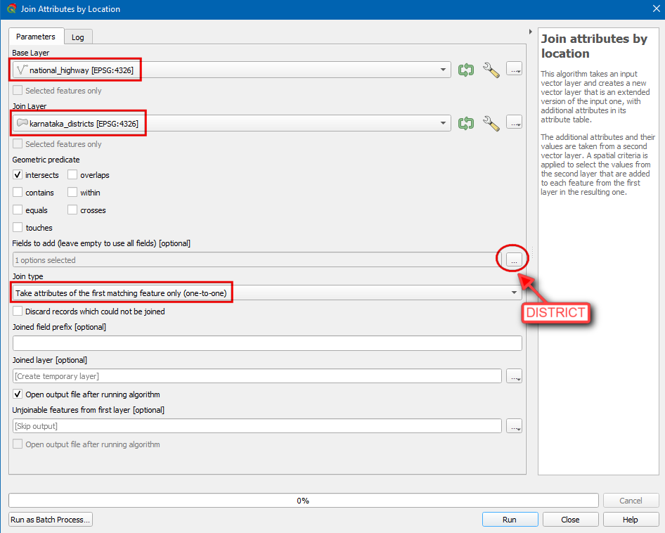
在karnataka_districts图层中有行政区划信息，但在national_highways中并没有。要在道路图层中添加行政区划名称信息，需要运行空间连接（spatial-join）。这要使用Join attributes by Location算法来实现。选择national_highways作为输入层，然后和karnataka_districts图层进行一对一连接。只选择DISTRICT域添加到输出上。

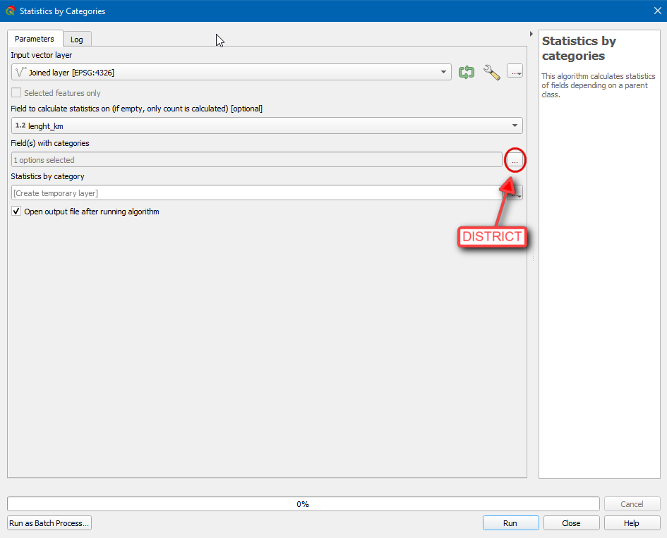
新的Joined layer图层就有了交叉的行政区划名存储在DISTRICT域中了。如果你用过之前版本的QGIS，你可能还记得当时需要调用插件Group Stats来实现这个功能。但现在可以通过内置的Statistic by Categories算法来实现了。选择Joined layer作为输入向量图层Input vector layer，选择length_km作为Field to calculate statistics on。选择DISTRICT作为Field(s) with Categories。

这个算法的输出结果是一个数据表，其中包含了对每个行政区在length_km列上的各种统计值。其中Sum 列的值就是各区的国家高速路总长度了。

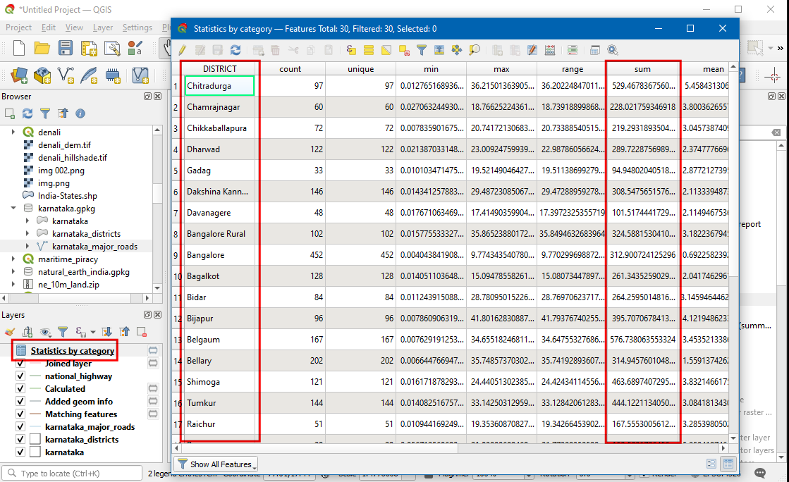
注意，这里我们所做的数据处理、空间分析和统计分析，都只是使用了处理算法，是一个快速、可重现、符合直觉的工作流。

了解更多

想要对处理工具箱（Processing Toolbox）中其他上千种工具有进一步了解，可以参考下面的视频。

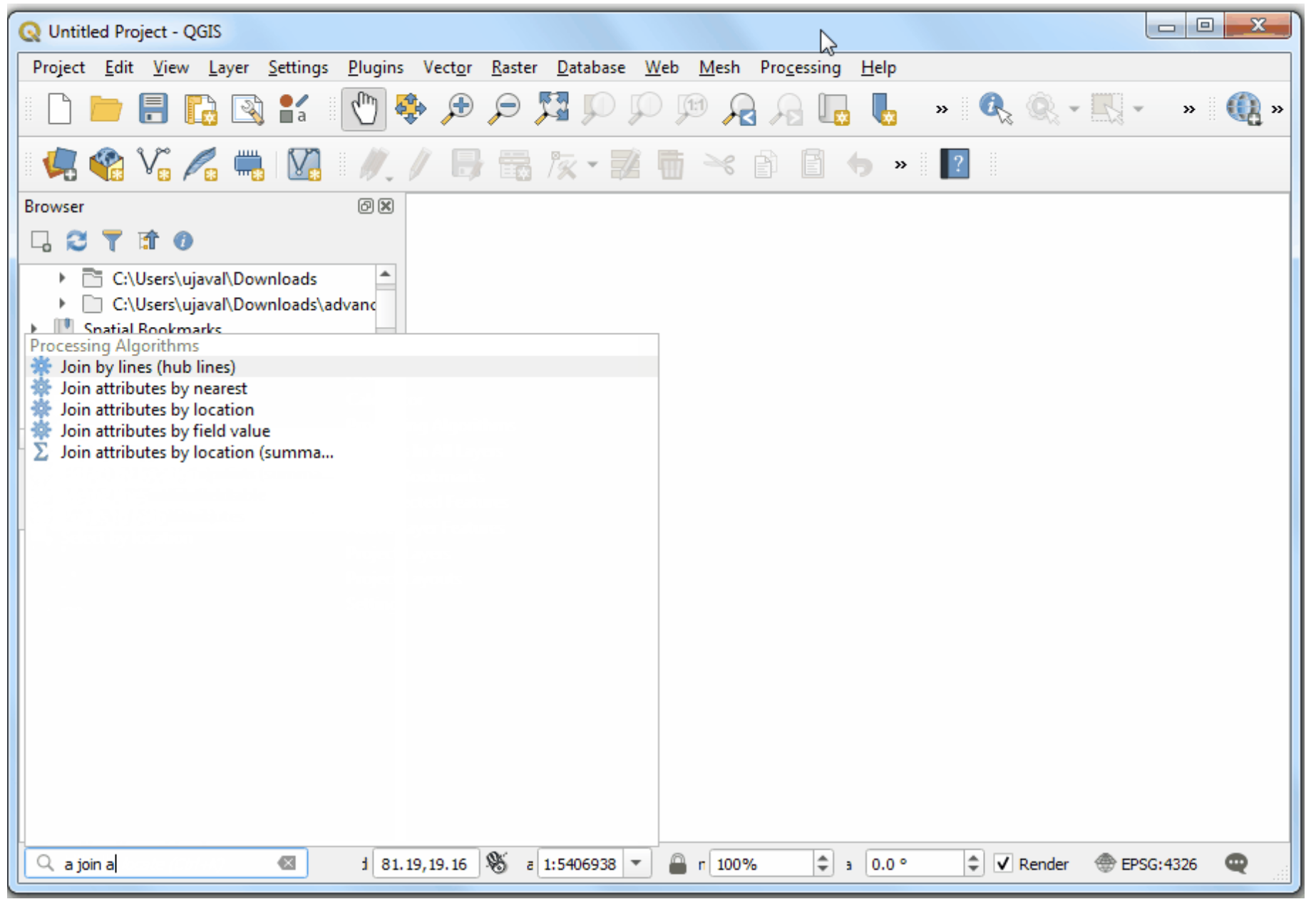
The Locator Bar

To take your processing experience to the next-level, you can use the built-in Locator Bar. At the bottom-left of QGIS main window, there is a universal search bar that can do keyword-search across layers, settings, processing algorithms and more. You can open the locator bar using the keyboard shortcut Ctrl+K.

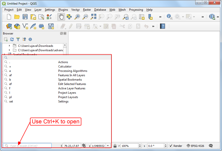
I find that rather than clicking-around the processing toolbox, you can just use the locator bar to search and open the algorithms. Type Ctrl+K, followed by a (to restrict search to algorithms), followed by a space and a few characters. Use the arrow keys to select and press Enter to open the algorithm.

View Animated GIF ↗

In-place Editing

Processing algorithms are designed to take inputs and produce outputs. The default behavior is to create a new layer after each operation. This is useful for many workflows, especially in an enterprise setting, where you may not have the ability to edit the source data. If your algorithms are altering the source data, that also means that the workflows cannot be reproduced easily. So you would want a setup where the algorithms read from source data and create modified outputs.

An exception to this workflow is when you are doing data editing. When your workflow involves creating new features or editing them - creating a new layer for every edit is undesirable. A recent QGIS crowd-funding campaign added the ability for processing algorithms to modify the features in-place and this functionality is available out-of-the-box in QGIS now.

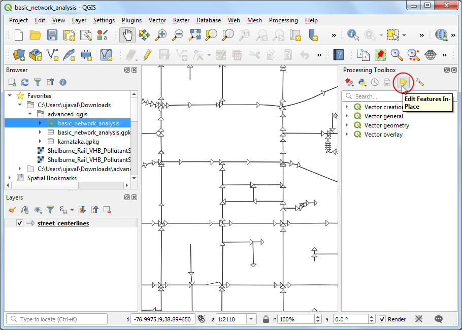
Load the basic_network_analysis project from the data package. This project contains a street network for Washington DC from DCGISopendata where the arrows display the digitizing direction of the line segments. You can click the Edit Features In-Place button in the processing toolbox to use algorithms that support this functionality. Once this mode is activated, processing algorithms will modify the selected features in the chosen layer instead of creating a new layer.

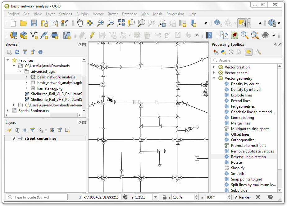
Select a line segment and run the Reverse line direction algorithm. The algorithm will enable editing on the layer, perform the operation and overwrite the existing feature with a segment in the reverse direction. You will see that the arrow rendering is now in the opposite direction.

View Animated GIF ↗

Batch Processing

So far we have run the algorithm on 1 layer at a time. But each processing algorithm can also be run in a Batch mode on multiple inputs. This provides an easy way to process large amounts of data and automate repetitive tasks.

The batch processing interface can be invoked by right-clicking any processing algorithm and choosing Execute as Batch Process.

练习: Clip multiple layers to a polygon

We will take multiple country-level data layers and use the batch processing operation to clip them to a state polygon in a single operation.

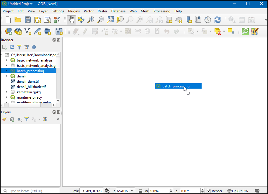
Open the batch_processing project.

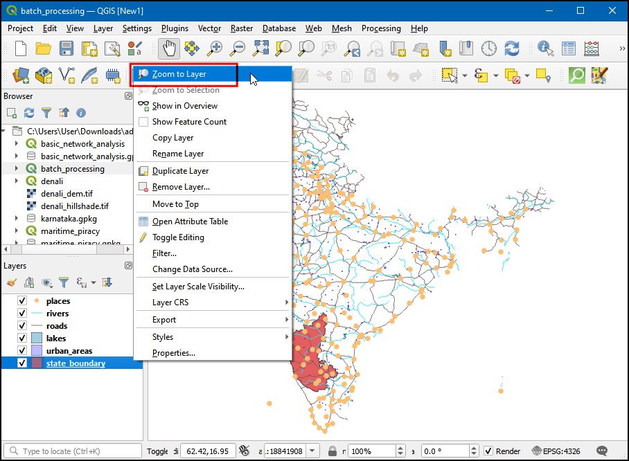
Next, right-click on the state boundary layer, and click Zoom to Layer.

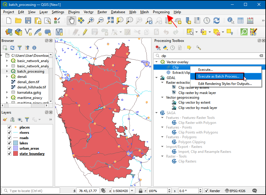
Now that we have centered on our area of interest, under the Processing menu and select toolbox. Now in Processing Toolbox, search for clip, under Vector overlay → Clip right-click and select Execute as Batch Process...

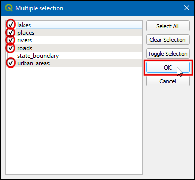
In the Batch processing - Clip dialog box, click the Autofill… under the Input layer column and choose Select from Open Layers...

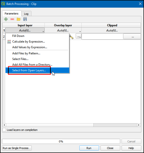
Select all data layers except state_boundary and click OK.

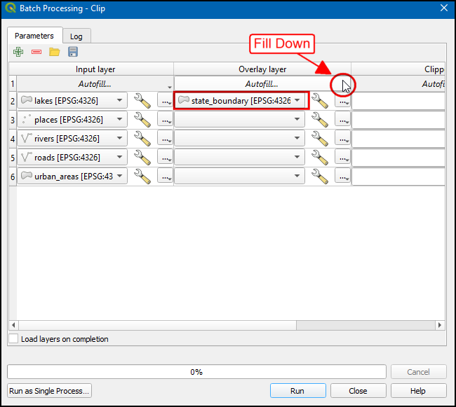
Under Overlay Layer select the state_boundary layer. Then click the drop-down button near Autofill… and choose to Fill Down. This will auto-populate all the Overlay Layer with the state_boundary layer.

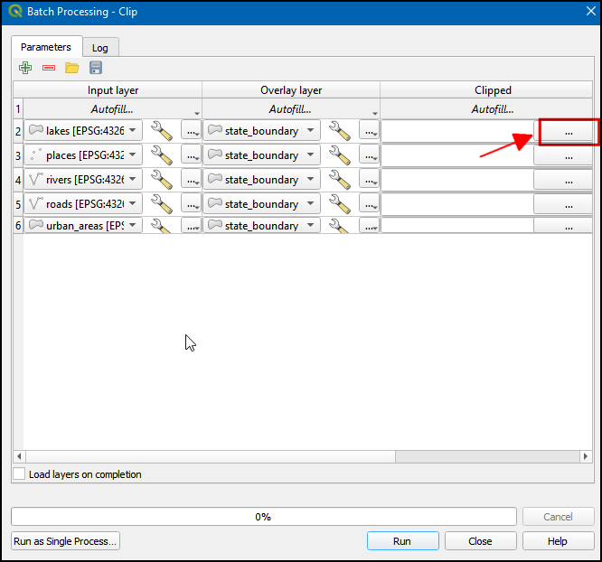
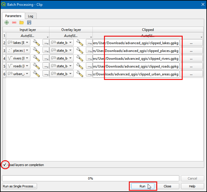
Under Clipped, select … button to add the output filenames.

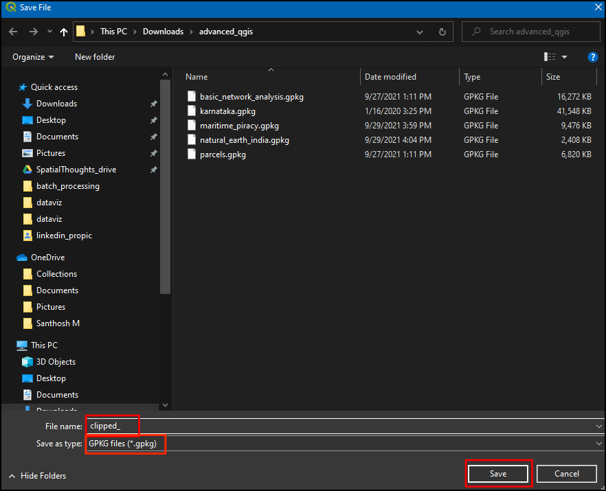
In the Save File dialog box, enter the File name as clipped_. This is just the prefix of the name that you will auto-complete in the next step. Select GPKG files (.gpkg) in Save as type. Click Save.

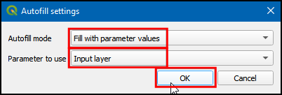
Next, you will be prompted to choose the Autofill settings. Select to Fill with parameter values as the Autofill mode, and Input layer as the Parameter to use. Click OK.

Note that each row has a different file name now. The output file name is the result of the chosen prefix and the autofill settings. Make sure the Load layers on completion box is checked and click Run.

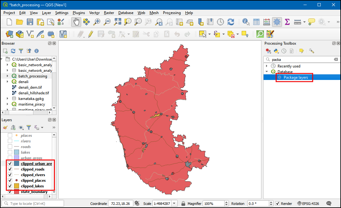
The resulting clipped layers will be added to the Layers panel. Turn off all previous layers in the Layers panel to see the results clearly. We can now combine all the clipped layers into a single geopackage file for ease of sharing. Now in the Processing Toolbox, search and select the Package Layers.

In the Package Layers dialog box, in Input layers choose all the clipped layers and in Destination GeoPackage click … and select Save to File…. Then save the file as clipped.gpkg. Click Run

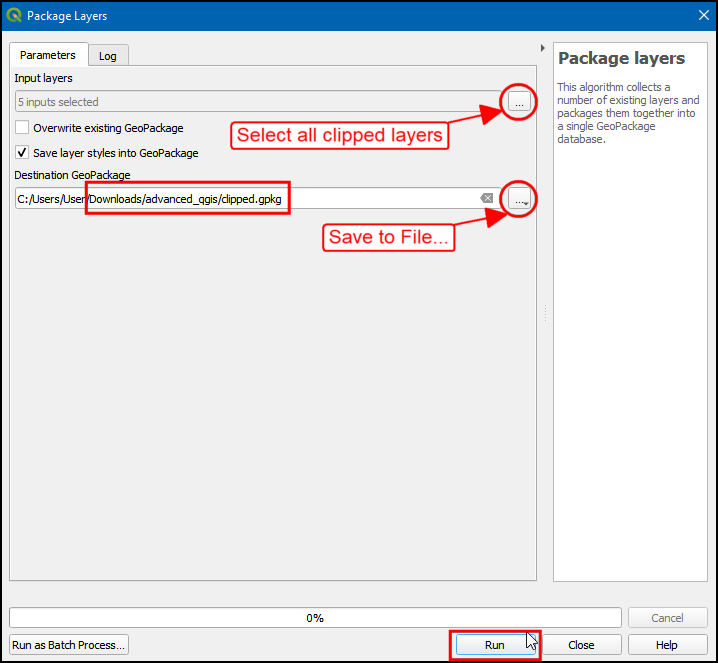
Now a new clipped.gpkg geopackage layer will be created with all the clipped layers in it.

Graphical Modeler

GIS Workflows typically involve many steps - with each step generating intermediate output that is used by the next step. If you change the input data or want to tweak a parameter, you will need to run through the entire process again manually. Fortunately, Processing Framework provides a graphical modeler that can help you define your workflow and run it with a single invocation. You can also run these workflows as a batch over a large number of inputs.

练习: Find the hotspots of piracy incidents

National Geospatial-Intelligence Agency’s Maritime Safety Information portal provides a shapefile of all incidents of maritime piracy in the form of Anti-shipping Activity Messages. We can create a density map by aggregating the incident points over a global hexagonal grid.

The steps needed to create a hex-bin layer suitable for visualization is as follows:

Reproject the input to an equal-area projection
Create a global hexagonal grid layer
Select all grids that intersect with at least 1 point
Count points within each grid

We will now learn how to build a model that runs the above processing steps in a single workflow.

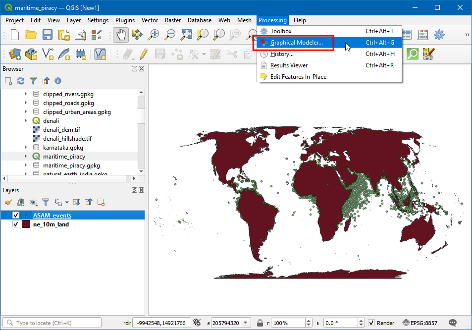
Open the maritime_piracy project.

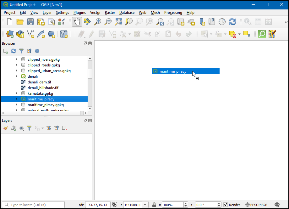
Launch the modeler from Processing → Graphical Modeler

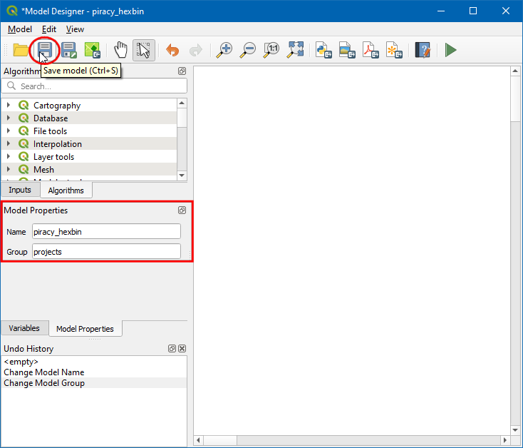
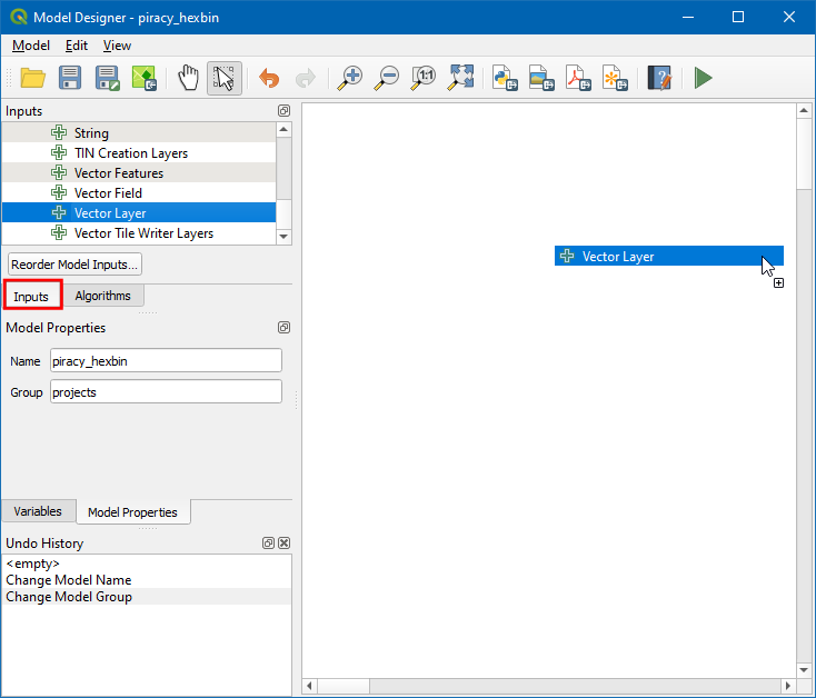
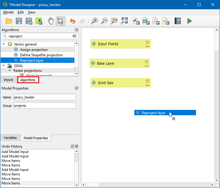
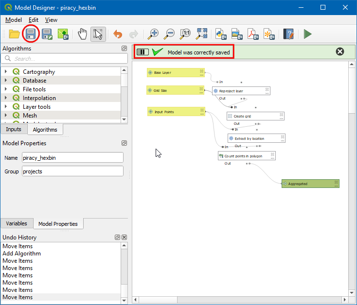
In the Processing Modeler dialog, locate the Model Properties panel. Enter piracy_hexbin as the Name of the model and projects as the Groups. Note that there is a History panel in the bottom left, which keeps track of all the work done in Model Builder. Click the Save button.

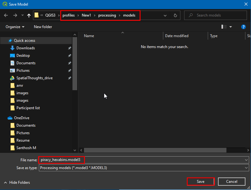
Save the model as piracy_hexbin.model3. Also, check the folder in which it is being saved. Processing → models, from this location QGIS will read the model by default.

Now, we can start building a graphical model of our processing pipeline. The Processing modeler dialog contains a left-hand panel and the main canvas. On the left-hand panel, locate the Inputs panel listing various types of input data types. Scroll down and select the + Vector Layer input. Drag it to the canvas.

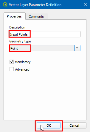
Enter Input Points as the Description and Point as the Geometry type. This input represents the piracy incidents point layer.

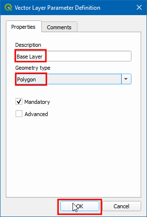
Next, drag another + Vector Layer input to the canvas. Enter Base Layer as the Description and Polygon as the Geometry type. This input represents the natural earth global land layer in which we will use as the extent of the grid layer.

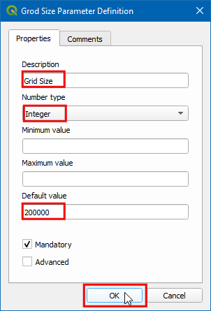
As we are generating a global hexagonal grid, we can ask the user to supply us with the grid size as an input instead of hard-coding it as part of our model. This way, the user can quickly experiment with different grid sizes without changing the model at all. Select a + Number input and drag it to the canvas. Enter Grid Size as the Parameter name, Integer as the Number Type, 200000 as Default Value, and click OK.

Now that we have our user inputs defined, we are ready to add processing steps. All of the processing algorithms are available to you under the Algorithms tab. The first step in our pipeline will be to reproject the base layer to the Project CRS. Search for the Reproject layer algorithm and drag it to the canvas.

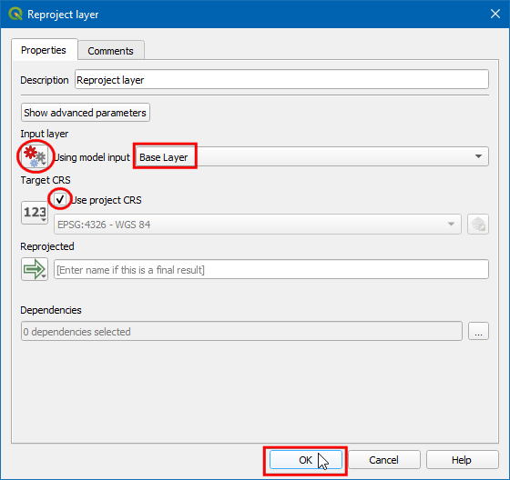
In the Reproject layer dialog, select Base Layer, by clicking the button under the Input Layer and select Model Input as the Input layer. Check the Use project CRS as the Target CRS. Click OK.

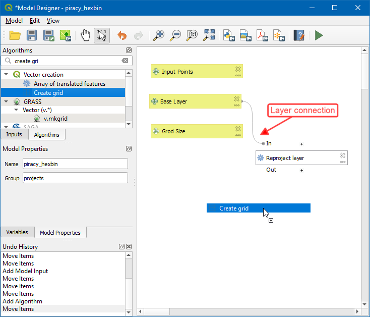
In the Processing Modeler canvas, you will notice a connection appear between the + Base Layer input and the Reproject layer algorithm. This connection indicates the flow of our processing pipeline. The next step is to create a hexagonal grid. Now search for the Create grid algorithm and drag it to the canvas.

In the Create grid dialog, choose Hexagon (polygon) as the Grid type. Select Algorithm Output by clicking the button under Grid extent and choose ‘Reprojected’ from the algorithm ‘Reproject Layer’ as the Grid extent.

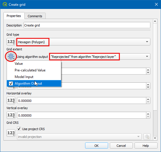
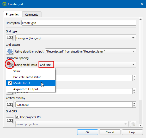
Select Model input by clicking the button under Horizontal Spacing and choose Grid Size as the Horizontal Spacing. Click OK.

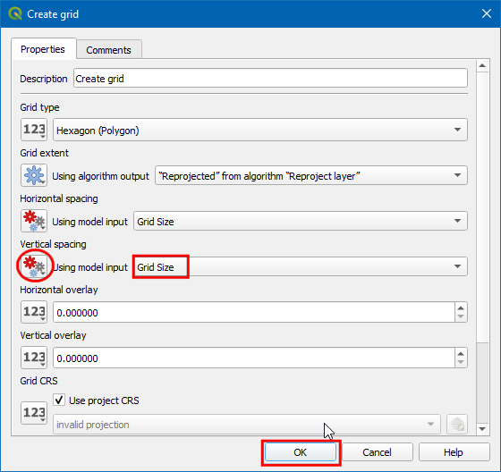
Select Model input by clicking the button under Vertical Spacing and choose Grid Size as the Vertical Spacing. Click OK.

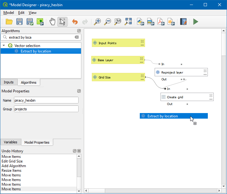
At this point, we have a global hexagonal grid. The grid spans the full extent of the base layer, including land areas and places where there are no points. Let us filter out those grid polygons where there are no input points. Search for Extract by location algorithm and drag it to the canvas.

Select Algorithm Output from the icon below Extract features from. Now choose ‘Grid’ from the algorithm ‘Generate Grid’. Click … at the right end.

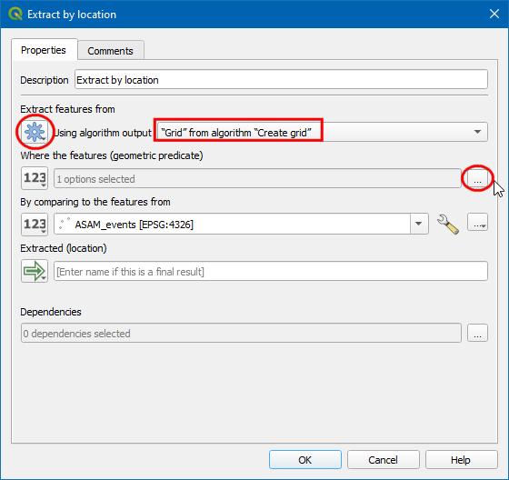
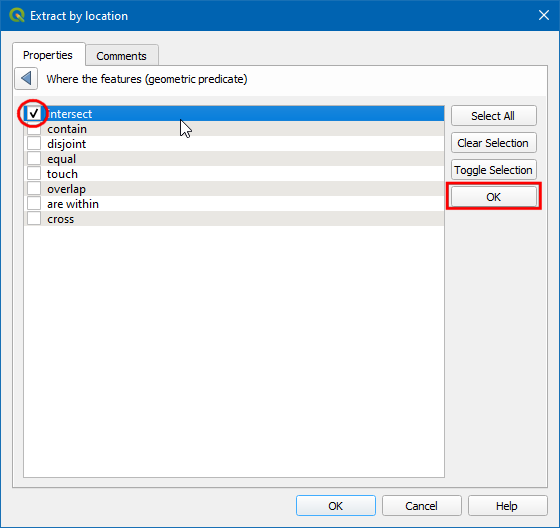
Select Intersect by clicking the button, as Where the features(geometric predicate). And click the triangle button to go back to the previous window. Now click OK.

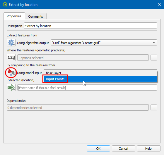
Select Model input by clicking the button under By comparing to the features from and choose Input Points as By comparing to the features from. Click OK.

Now, we have only those grid polygons that contain some input points. To aggregate these points, we will use Count points in polygon algorithm. Search and drag it to the canvas.

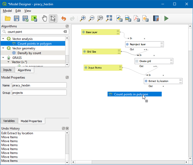
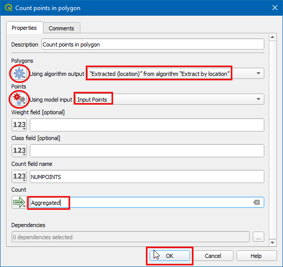
Select Algorithm Output by clicking the button under Polygons and choose ‘Extracted (location)’ from algorithm ‘Extract by location’ for Polygons. Now, Select Model Input by clicking the button under Points and choose Input Points for Points. Type NUMPOINTS in Count field name. At the bottom, name the Count output layer as Aggregated. Click OK.

The model is now complete. Click the Save button. If the model is saved, then a green notification will pop on the screen.

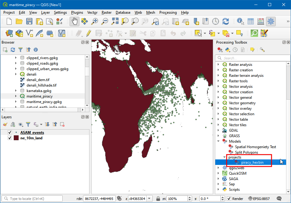
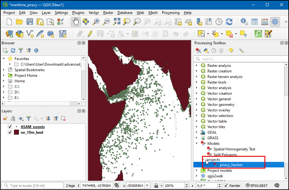
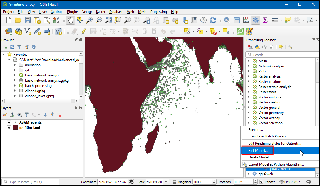
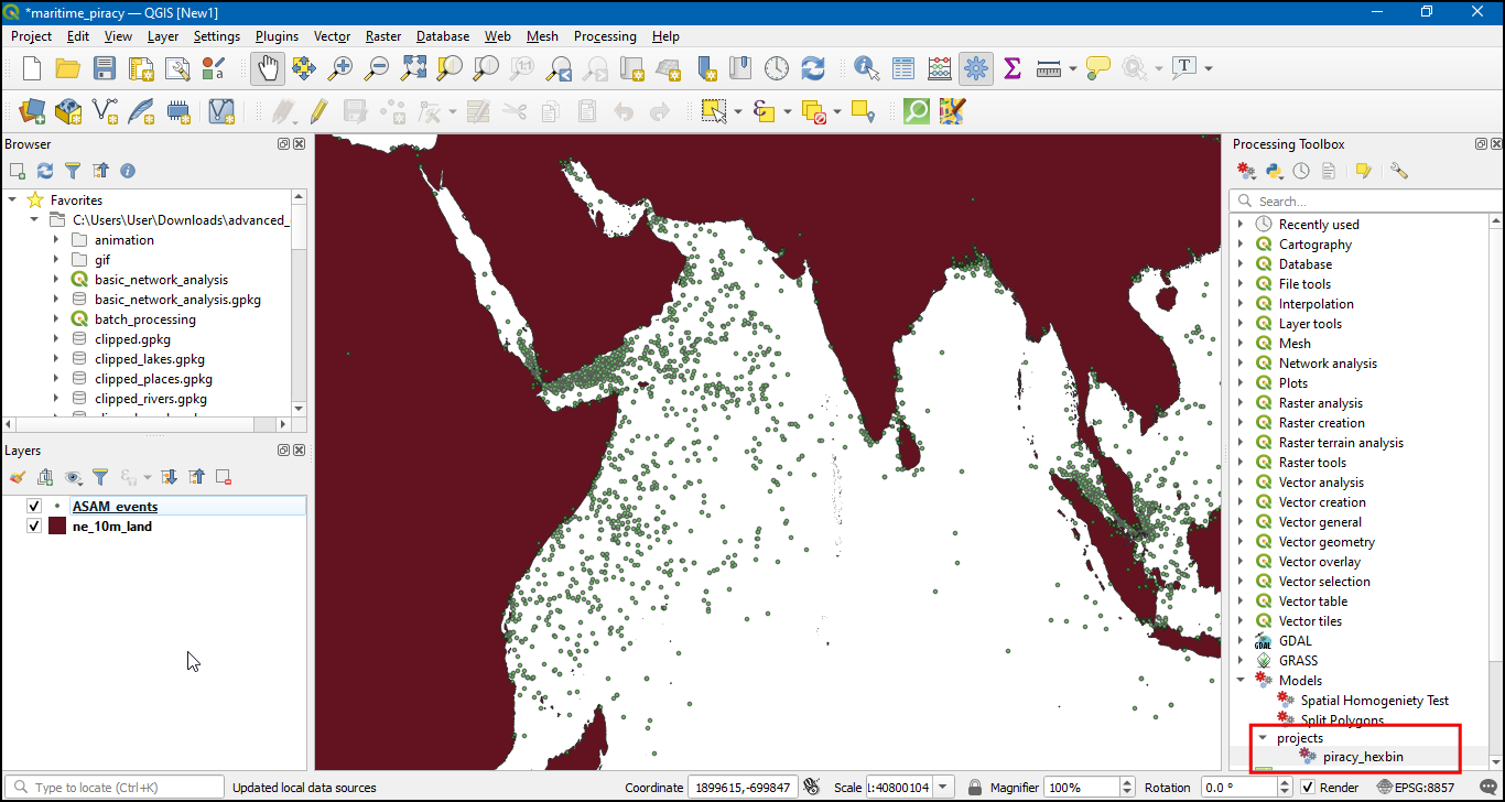
Switch to the main QGIS window. You can find your newly created model in the Processing Toolbox under Models → projects → piracy_hexbin. Double-click to run the model.

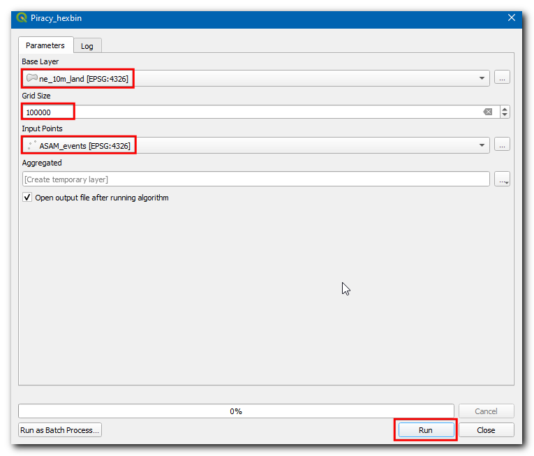
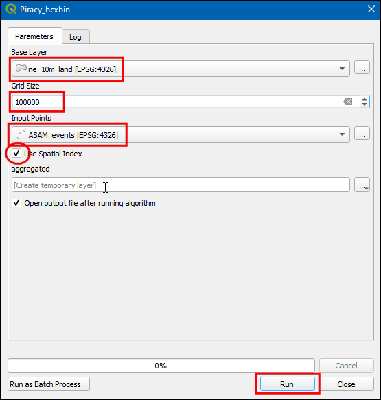
Our Base Layer is the ne_10m_land and the Input Points layer is ASAM_events. The Grid Size needs to be specified in the units of the selected CRS. Enter 100000 as the Grid Size. Grid size is in the unit of the current CRS, which is meters. Click Run to start the processing pipeline. Once the process finishes, click Close.

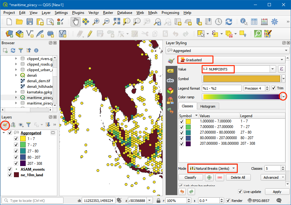
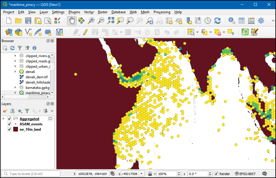
You will see a new layer Aggregated loaded as the result of the model. As you explore, you will notice the layer contains an attribute called NUMPOINTS containing the number of piracy incidents points contained within that grid feature. Let’s style this layer to display this information better. Click the Open Layer Styling Panel button from the Layers panel. Select Graduated symbology and NUMPOINTS as the Column. Click the dropdown next to the Color ramp and select the Viridis ramp. Click the dropdown again and select Invert Color Ramp to reverse the order of color. The Graduated symbology will divide the values in the selected column into distinct classes and assign a different color to each of the classes. Select Natural Breaks (Jenks) as the Mode and click Classify.

We will use a clever trick to make the visualization better. We can use QGIS variables to set the edges of the hexagon with a slightly darker shade of the fill color. Click on the Symbol. Click Simple Fill. Click the Data defined override button next to Stroke color and select Edit.

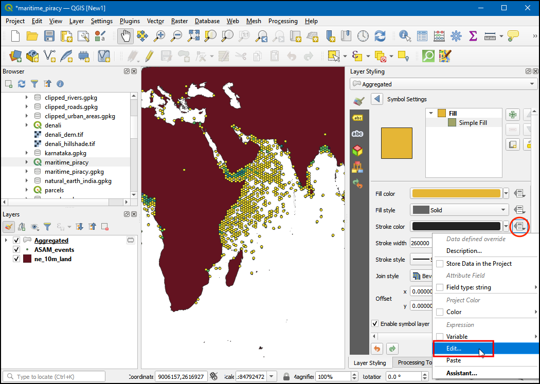
Enter the following expression to set the stroke color to 30% darker than the fill color and click OK. The map rendering will change to a much smoother visualization.

darker( @symbol_color , 130)

Challenge: Improve the model

Can you change the model so that instead of entering the grid size in meters, the user can enter the size in kilometers?

Hint: The Create Grid algorithm expects the size in meters, so you will have to convert the input to meters.

Spatial Indexing

When you ran your model, you may have noticed a warning message No spatial index exists for the input layer, performance will be severely degraded. This is because certain spatial queries make use of a spatial index and QGIS warns you when having a spatial index can speed up your operations. PostGIS documentation has a good overview of spatial indexes and why they are important.

You can compare a spatial index to a book index. When you want to search for a particular term, rather than scanning each page sequentially, you can speed up your search by looking up the index and directly going to the pages where the word appears. Spatial indexes work in similarly. You spent the effort once to create the index and all subsequent operations can make use of it. When you create a spatial index, each feature’s bounding box is used to establish its relationship with other features. This is stored alongside the dataset and can be used by algorithms. When trying to determine spatial relationships, the algorithms speed-up the look-up using the following two-pass method:

Step 1: Use the spatial index to determine which target features’ bounding boxes intersect with the source feature’s bounding box. Since the spatial index already has computed this - this is very fast. The result is a list of candidate features.
Step 2: Now that there is a small subset of candidate features, iterate over them and use their full geometry to evaluate exact intersections.

For large datasets, this approach helps reduce the processing time significantly.

查看幻灯片

QGIS has built-in tools to create and use spatial indexes. Let’s see how we can create a spatial index for a layer and use it in our model.

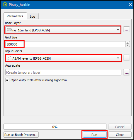
Double click on the piracy_hexbin model from Processing Toolbox, select ne_10m_land as Base Layer, 200000 as Grid size and ASAM_events as Inputs Points. Click Run.

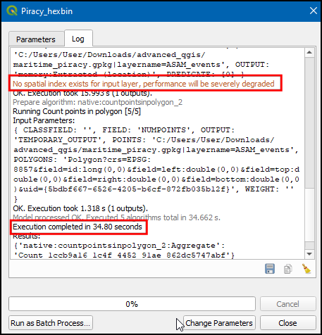
Switch to Log, and note down the execution time of the model. In this instance we got 34.80 seconds (The exact time will vary depending on your computer configuration). Also note that it prompts a warning No spatial index exists for input layer, performance will be severely degraded.

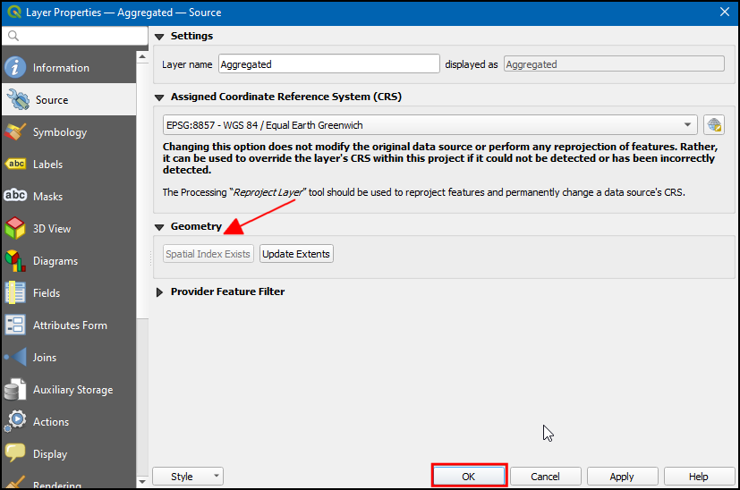
To create spatial index right-click the Aggregated layer and select Properties.

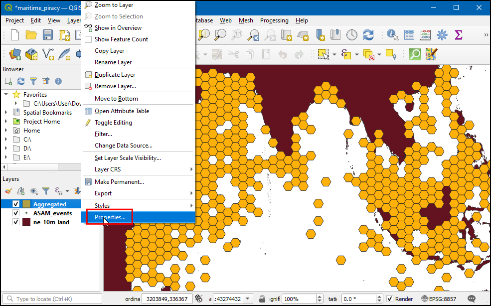
In the Layer Properties dialog, switch to the Source tab. You will see the Create Spatial Index button. This button indicates that this layer does not currently have a spatial index. Click that button to create a spatial index. But we will use a better and more scalable way. Click OK and close the Layer Properties dialog.

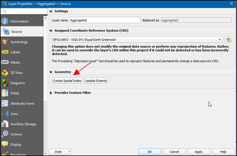
Go to Processing → Toolbox. Search for the algorithm Vector general → Create spatial index and double-click to launch it.

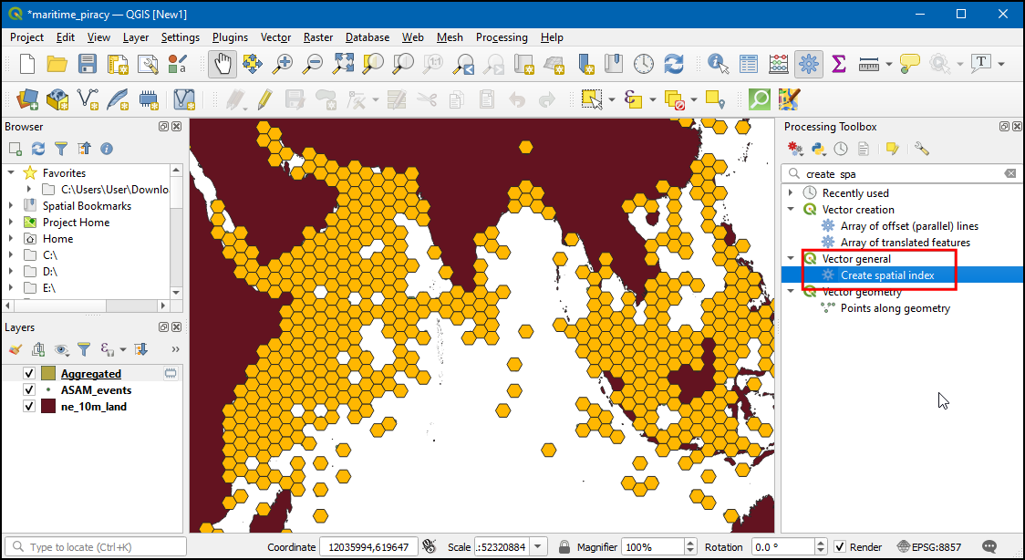
Select Aggregated layer as the Input layer and click Run.

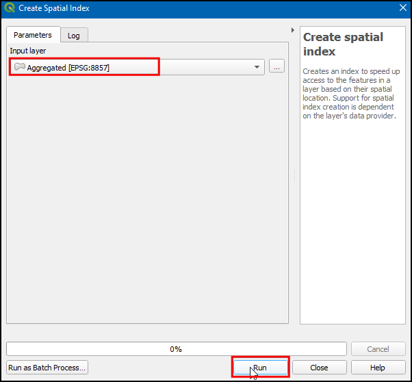
Creating a spatial index is usually a fast operation. Once the algorithm finishes, right-click on the Aggregated layer and select Properties. Switch to the Source tab and you will see that the button has now changed to Spatial Index Exists - indicating that the layer now has a spatial index.

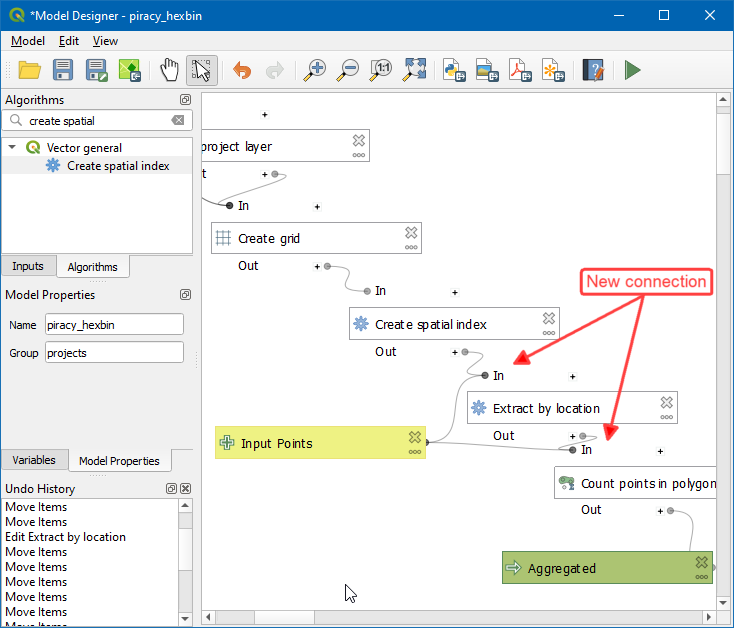
While creating a spatial index on a layer like this is useful, it is even more powerful to have the spatial index created during the execution of our model. We will see how to add the spatial index creation step in our model. Right-click the piracy_hexbin model and select Edit Model…. Search Create spatial index in Algorithms tab and drag it to the model canvas.

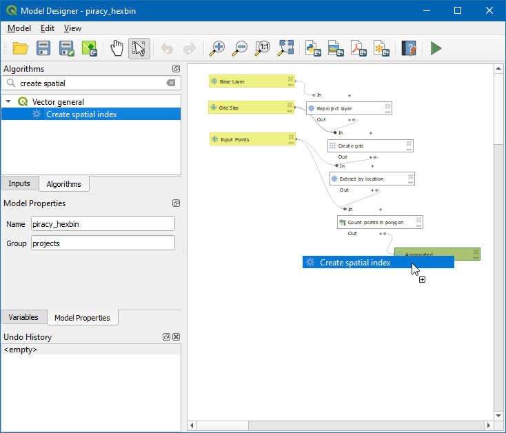
Choose Algorithm output from the button below Input Layer, and select “Grid” from algorithm “Create Grid”. Click OK.

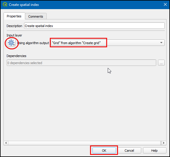
You will see that the newly added Create spatial index algorithm is connected to the Create grid algorithm. But the workflow should be, Create grid → Create spatial index → Extract from location.

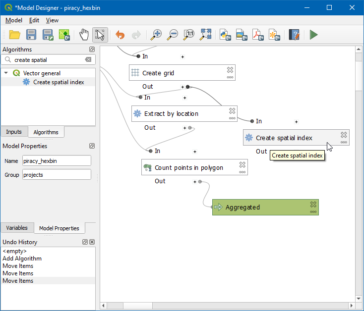
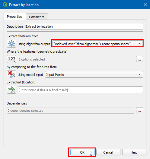
Right-click the Extract by location layer and select Edit. In Extract features from select “Indexed Layer” from algorithm “Create spatial index”.

Now you will see the model diagram updated and the connection changed between the Create Grid and Extract by location layer. Click Save model.

Now return to the main canvas and select piracy_hexbin model.

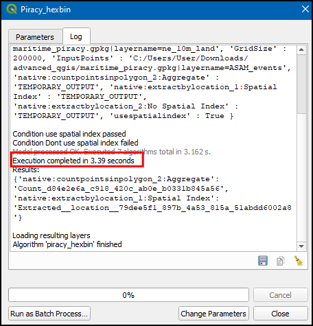
Select ne_10m_land as Base Layer, 200000 as Grid size and ASAM_events as Inputs Points. Click Run.

In this instance we got 3.39 seconds (The exact time will vary depending on your computer configuration). Also, note that it has executed 5 algorithms which is including creating the spatial index.

Conditional Branching

A key feature introduced in QGIS 3.14 was the ability for models to have a conditional branch. This allows models to check for a condition and execute a different part of the model based on the output of the condition. This is equivalent to If/Else statements in a programming language.

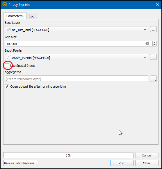
Let us develop a Conditional branch in the piracy_hexbin model. We will add a new check-box input Use Spatial Index - that allows the user to specify whether to use a spatial index in the model. We will add a conditional branch that takes the following actions:

If the Use Spatial Index option is selected, the model will create a spatial index for the grid layer and use it in the subsequent steps.
If the option is not selected, the model will proceed without generating a spatial index.
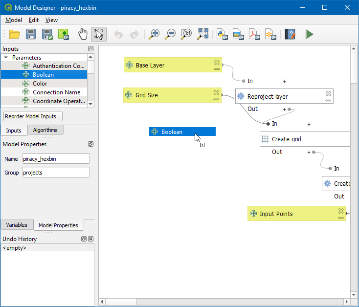
Right-click the piracy_hexbin model and select Edit Model….

Search for +Boolean in Inputs tab and drag to canvas.

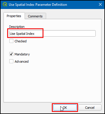
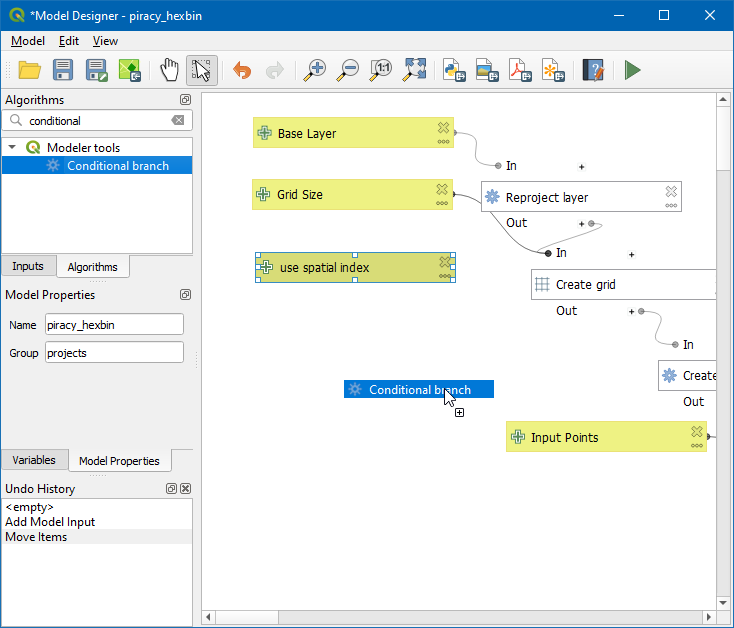
Give Description as Use Spatial Index, leave Checked unticked. Click OK.

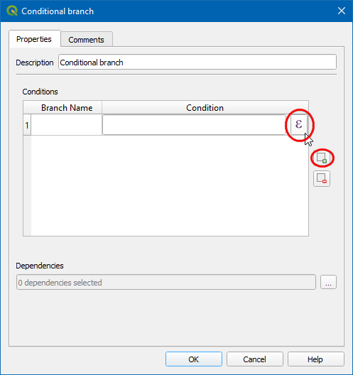
Now, search for Conditional branch in Algorithms tabs and drag to canvas.

Click the Add button and select the Expression Dialog button.

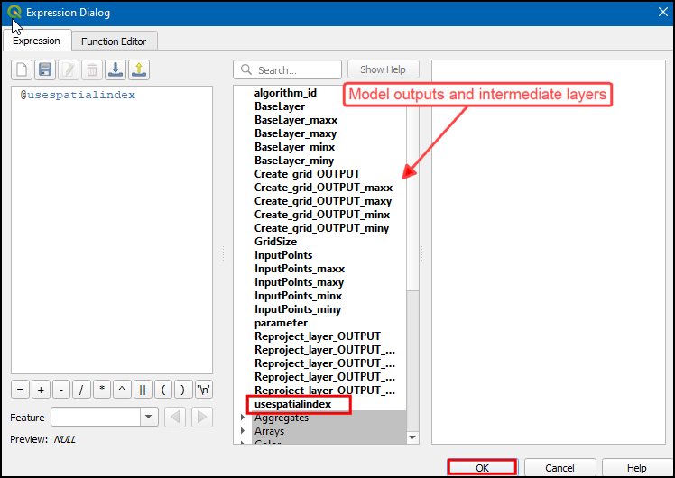
6. All the model output and intermediate layers will be displayed in Bold characters, double click in usespatialindex. It will add the variable @usespatialindex as the expression. Click OK.

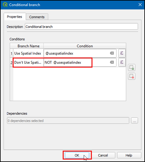
Now, in Branch Name type Use Spatial Index. We will add another branch now. Click the Add button and enter the Branch Name as Don’t Use Spatial Index. Since this is the opposite condition, we can use the expression NOT @usespatialindex Click OK.

Make sure to hit the Enter key after typing the Branch Name. The input may not be saved if you forget to do so.

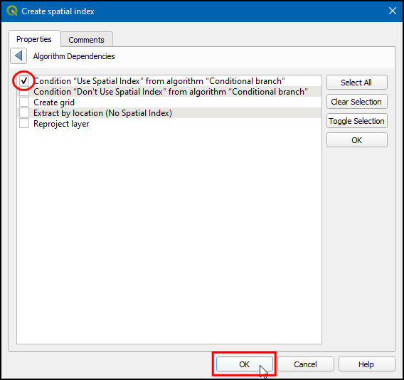
We have 2 branches in the model. Let’s connect them to appropriate algorithms. Double click on Create spatial index algorithm in model canvas and click … next to Dependencies.

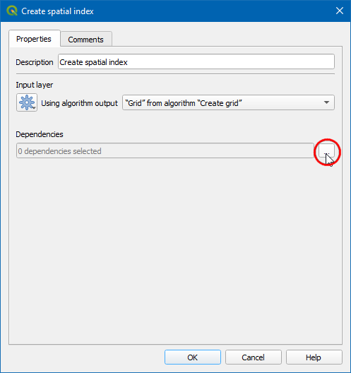
Choose Condition “Use Spatial Index” from algorithm “Conditional branch” and click OK. The Use Spatial Index branch is now ready. Let’s build the other branch.

Search for Extract by location in Algorithms tab and drag to canvas.

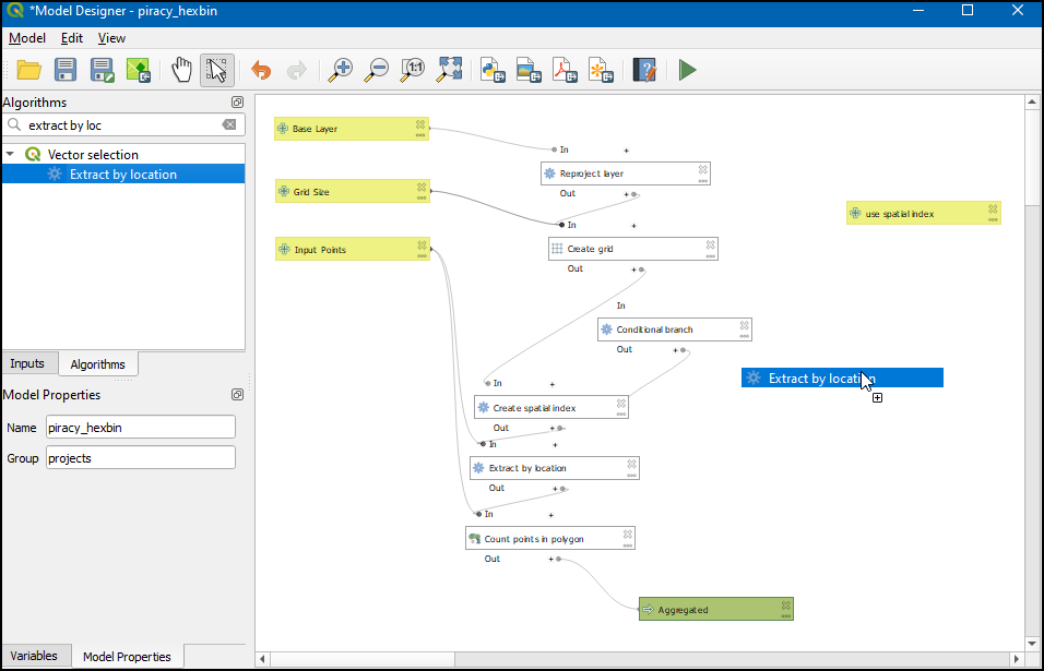
In the Description type Extract by location (No Spatial Index). Choose Algorithm Output in Extract features from and select “Grid” from algorithm “Create grid”. Click … next to Dependencies.

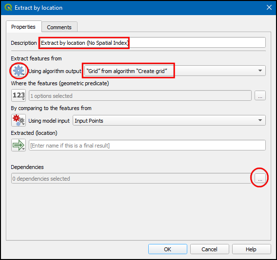
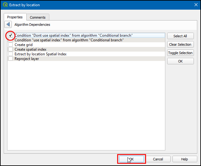
Choose Condition “Dont use Spatial Index” from algorithm “Conditional branch”. Click OK.

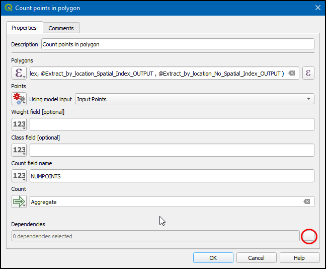
Similarly in Extract by location using Spatial Index change the description to Extract by location (Spatial Index). Both the branches will be executed according to the user selection whether to use the spatial index or not. The next step is to update the the Count points in polygon algorithm to use the appropriate output. Double-click on the algorithm box.

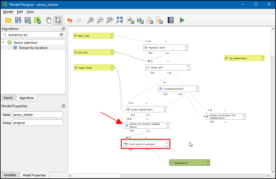
Under Polygons change Algorithm output to Pre-calculated Value, then press the Expression button.

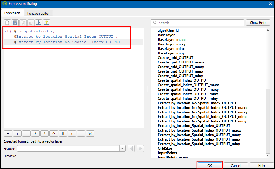
In the Expression Dialog, we need to select output from any one of the Extract by location algorithms based on the user condition of @usespatialindex. We can use the if condition to return a layer based on user input. Use the expression below. Remember to pick the variables from the list and double-click them to enter them in your expression. If you had named the algorithms or input differently, the variable names will be different for you. Click OK.

if( @usespatialindex ,  
    @Extract_by_location__Spatial_Index__OUTPUT ,
    @Extract_by_location__No_Spatial_Index__OUTPUT)

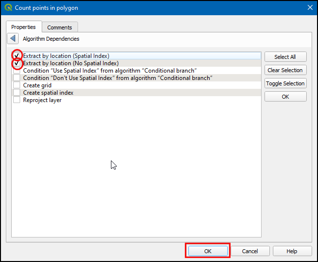
Now click … in Dependencies.

Check Extract by location (Spatial Index) and Extract by location (No Spatial Index) and click OK.

Now that the model is completed, click Zoom full button to view the model. Let us save the model click Save model button.

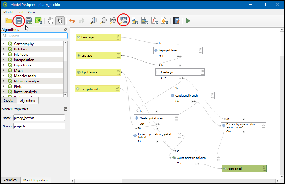
Now in the Processing toolbox, under that Models → projects → piracy_hexbin model will be available. Double click to execute it.

In the Base Layer select ne_10m_land, Grid size as 100000, and Input points as ASAM_events, check Use Spatial Index and click Run.

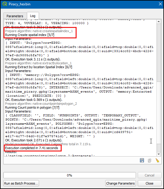
Switch to Log, we can notice the Create spatial index algorithm is activated, and the total time of execution is 7.41 seconds.

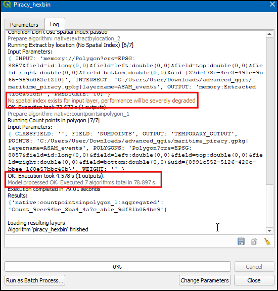
Now switch to Parameters, un-check the Use Spatial Index and click Run. tab.

Switch to the Log, we can notice the No spatial index exists for input layer, performance will be severely degraded warning get displayed, and the execution took 78.897 seconds.

Enabling Reproducible Workflows

To ensure that you are always able to reproduce your results, it is recommended to bundle the model in your project. The modeler interface has a button Save model in project that will embed the model in your QGIS project file.

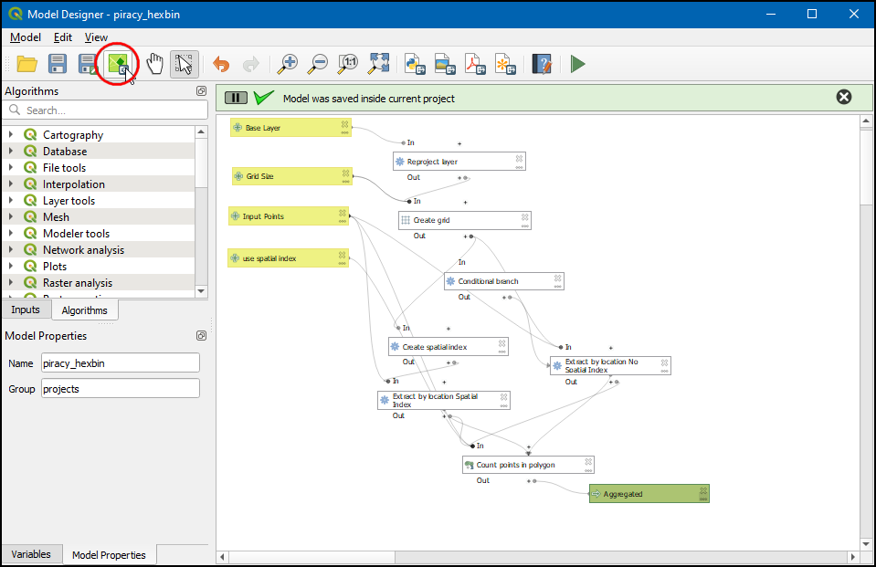
Once the model is embedded, Whenever you open the project, the model will be available to the user under the Project models in the Processing Toolbox.

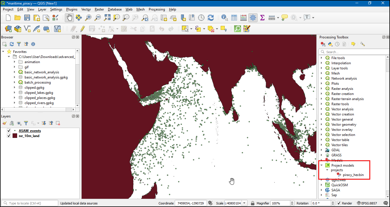
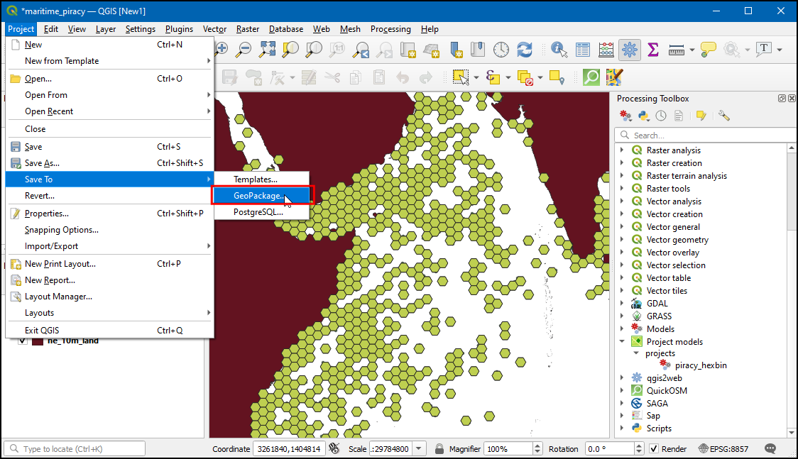
Now, lets save this project in martime_piracy.gpkg geopackage. Click Project → Save To → GeoPackage….

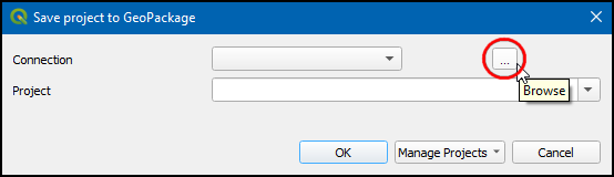
In the Save project to GeoPackage dialog box, click … to browse to martime_piracy geopackage.

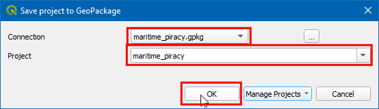
Enter project name as martime_piracy and click OK.

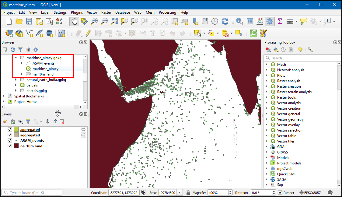
Now in Browser, under martime_piracy.gpkg the project is saved. You now have just 1 GeoPackage file that contains all your input layers, styles, project and models. Sharing this 1 file will enable anyone to reproduce your output using the embedded model and layers.

2D Animations

Time is an important component of many spatial datasets. Along with location information, time providers another dimension for analysis and visualization of data. If you are working with a dataset that contains timestamps or have observations recorded at multiple time-steps, you can easily visualize it using the Temporal Controller in QGIS 3.14 or above.

练习: Create a GIF showing changes in piracy hotspots over time

We will continue to work with the maritime piracy dataset. First, we will create a heatmap visualization and then animate the heatmap to show how the piracy hot-spots have changed over the past 2 decades.

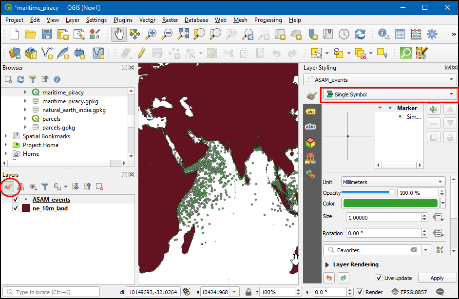
Open the maritime_piracy project from the data package. There are thousands of incidents and it is difficult to determine with more piracy. Rather than individual points, a better way to visualize this data is through a heatmap. Select the ASAM_events layers and click the Open the layer Styling Panel button in the Layers panel. Click the Single symbol drop-down.

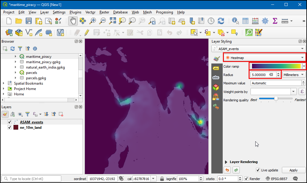
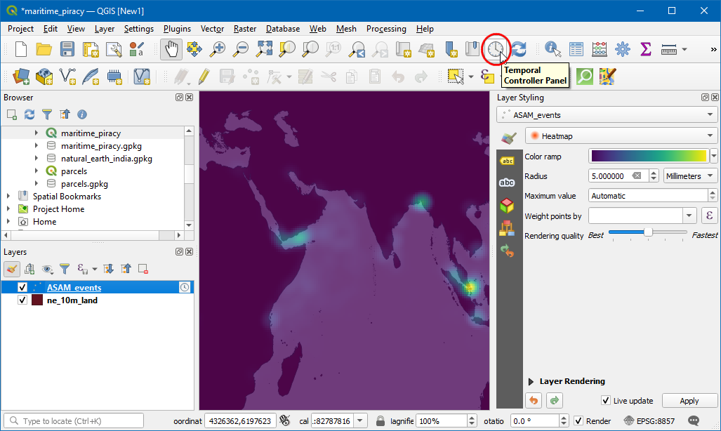
In the renderer selection drop-down, select Heatmap renderer. Next, select the Viridis color ramp from the Color ramp selector. Adjust the Radius value to 5.0. At the bottom, expand the Layer Rendering section and adjust the opacity to 75.0%. This gives a nice visual effect of the hotspots with the land layer below.

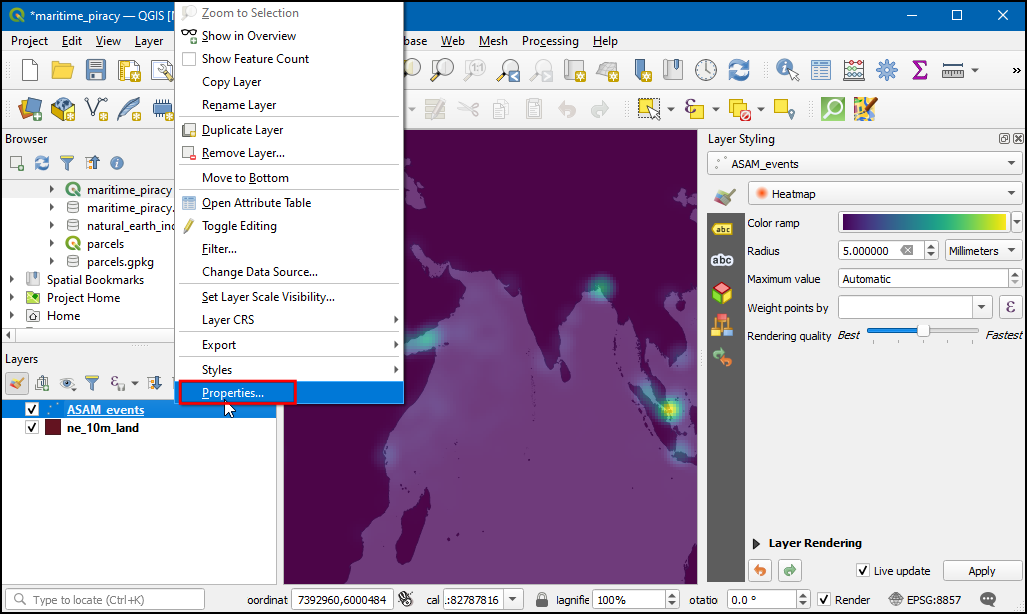
Now let’s animate this data to show the yearly map of piracy incidents. Right click on ASAM_event layer, and choose Properties.

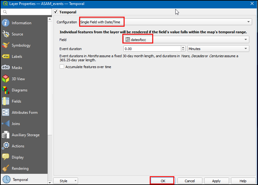
In the layer properties dialog box, select the Temporal tab and enable it by clicking the checkbox.

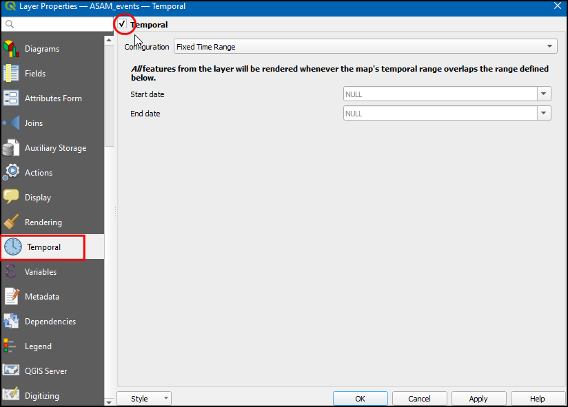
The source data contains an attribute dateofocc - representing the date on which the incident took place. This is the field that will be used to determine the points that are rendered for each time period. Select Single Field with Data/Time in Configuration Drop down menu, dateofocc as Field. Click OK.

Now a Clock symbol will appear next to the layer name. Click on the Temporal Control Panel (Clock icon) from Map Navigation Toolbar.

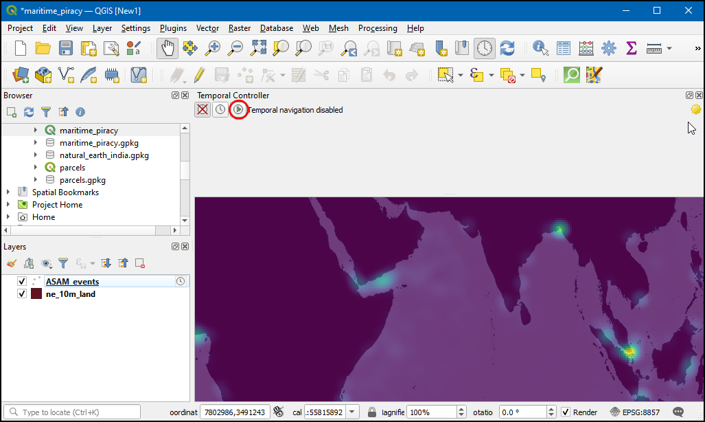
Click on the Animated Temporal Navigation (play icon).

By default, the date range is set to the current date. Click Set to Full Range button to set the date range from the dataset.

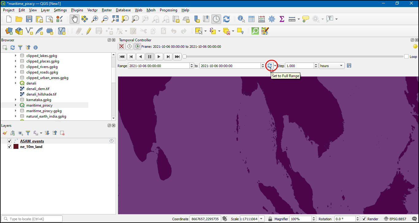
Now the data will be set to 2000-01-02 to 2018-01-01. We want to create an animation showing yearly changes to the hotspot. Set the Step to years. Click play button to start rendering.

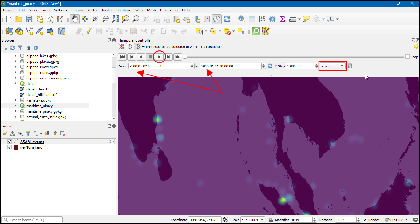
It will be useful to add a label to the animation showing the date of the animation frame being displayed. We can use the Title Decoration to place that label. Go to View → Decorations → Title Label Decorations. Click the checkbox to enable it and then the Insert an Expression button.

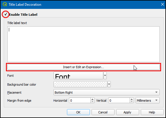
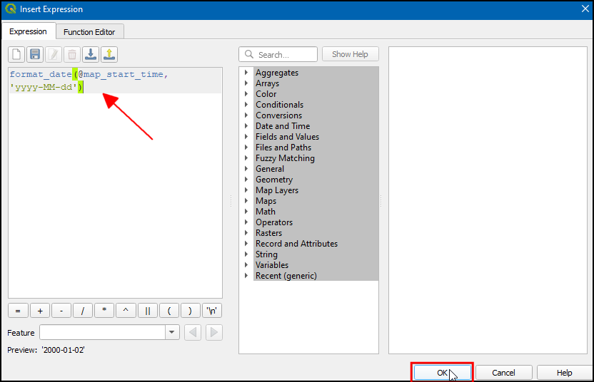
Enter the following expression to display the year and click OK.

format_date(@map_start_time, 'yyyy-MM-dd')

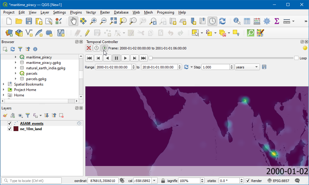
Select font size as 25, set background color as white. In placement choose Bottom Right. Now click OK.

View Animated GIF ↗

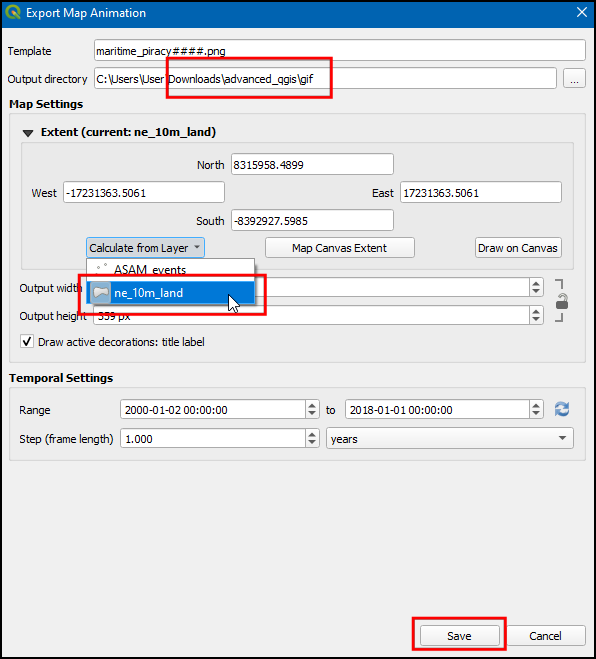
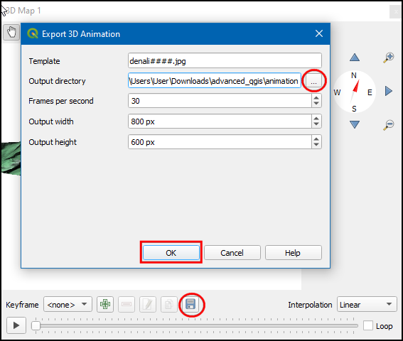
Once the parameters are set accordingly, the date will displayed on the map. To export these as images and convert them as GIF select the Export Animation (save icon) in the Temporal controller window.

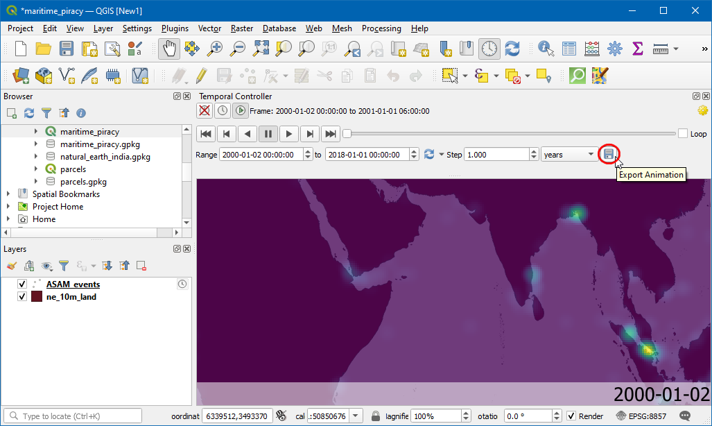
Choose the directory to save the images and select the ne_10_land for map extent.

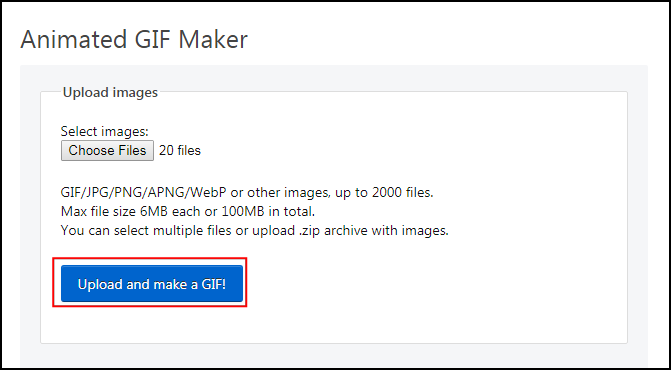
Once the export finishes, you will see PNG images for each year in the output directory. Now let’s create an animated GIF from these images. There are many options for creating animations from individual image frames. We like [ezgif.com] for an easy and online tool. Visit the site and click Choose Files and select all the .png files. You may want to sort the images by Type to allow easy bulk selection of only .png files. Once selected, click the Upload and make a GIF! button.

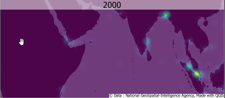
Challenge: Improve the animation

You will notice that for each frame of the animation, the year is displayed at the top-center. But instead of the full date and time, let’s change it to display the year that the map represents. Also, place the copyright info at the bottom right. The output should look something like below.

View Animated GIF ↗

3D Animations

Recent versions of QGIS include native support for 3D data. Using this feature, you can easily view, explore and animate 3D elevation data. Note that your computer must have a supported graphics card for this feature to work.

练习: Create a 3D Flythrough

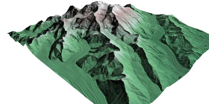
We will work with a 5m Digital Elevation Model (DEM) of Denali peak in Alaska and create an animation showing a 3D visualization of the dataset.

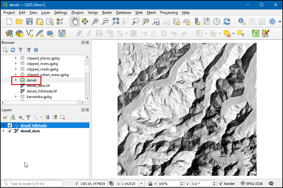
Open the denali project from the data package. The data contains the raw DEM layer and a hillshade layer created from the DEM.

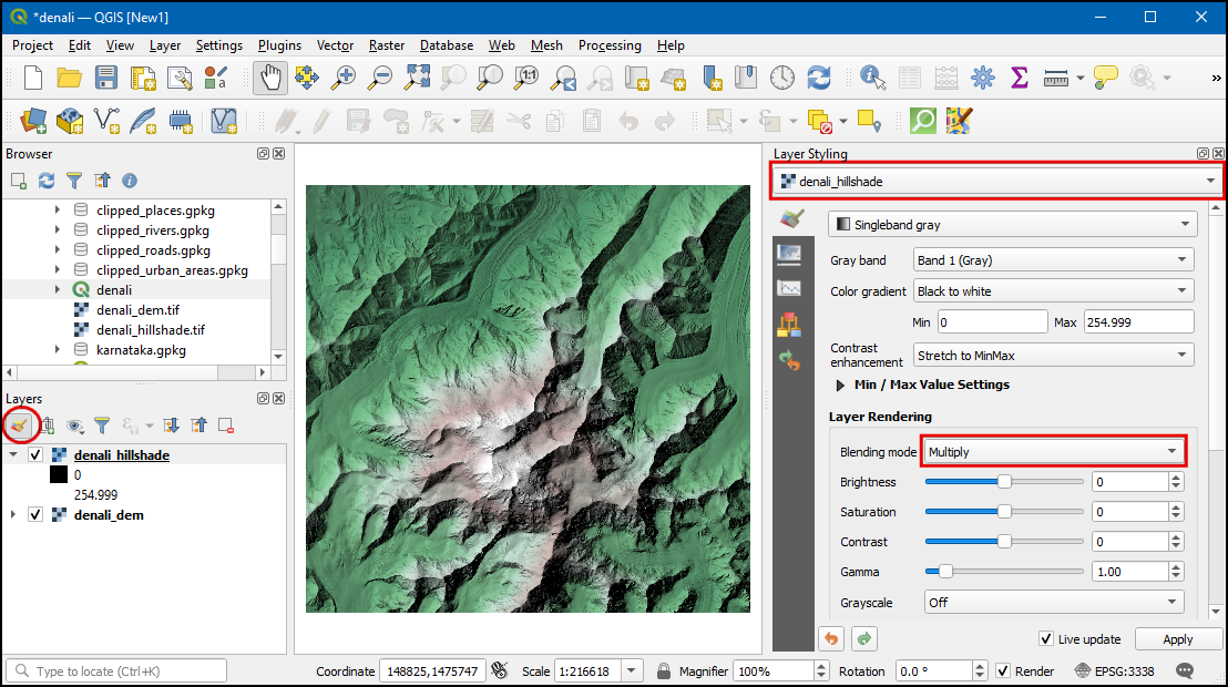
Let’s create a colorized hillshade. It is possible to drape an image or colorized DEM to a hillshade layer using QGIS’s Layer Blending Modes. Click on the Open the Layer Styling Panel icon. In the Layer styling panel, choose denali_hillshade and under Layer Rendering choose Multiply as Blending mode. The selected layer will be blended with the bottom layer. This is a great way to visualize your elevation dataset.

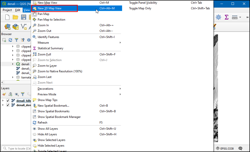
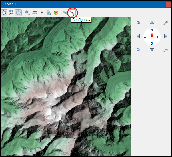
Let’s view this data in 3D. Go to View → New 3D Map View.

A new map window will open containing the rendered map layers from the main canvas. Click the Configure button.

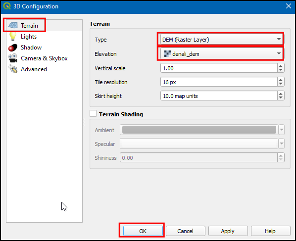
In the Terrain section, select DEM (Raster Layer) as the Type. Select denali_dem layer as the Elevation. Click OK.

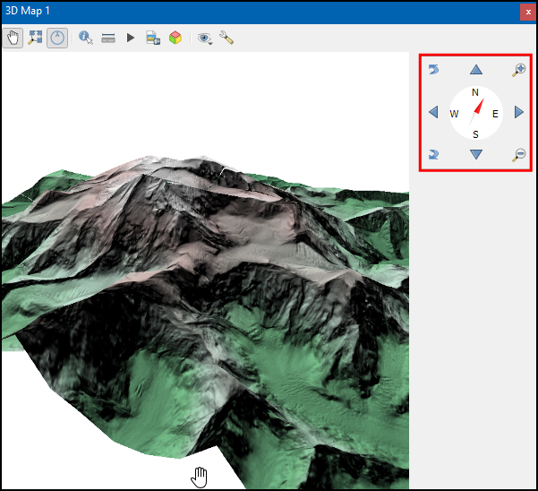
In the 3D view, you can hold the Shift key and drag your mouse to tilt the top-down view. You will see the map in 3D. You can also use the controls on the right-hand panel to tilt, zoom and pan the view.

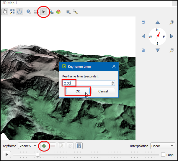
Now we will create an animation. Click the Animations button in the toolbar. To animate the view, we must define certain keyframes. Once you define a specific view for keyframes at different times, the system will try to smoothly animate the views between them. You can use the slider to go to a specific time, use the controls to set a specific view and click the + button to add a keyframe. Click the Play button to see the animation in action.

Once you are satisfied, click the Export Animation Frames button. Choose an output directory on your computer and click OK. Individual frames will be rendered and saved as separate files.

As we did in the previous section, you can use a service such as ezgif.com to create a GIF/Video from these frames.

View Animated GIF ↗

Summary Aggregate Expressions

QGIS expression engine has a powerful function called ‘summary aggregates’ that allows evaluating a feature’s geometry and attributes with those of another layer. Expressions can be used for static calculations as well as on-the-fly computations, such as labels, virtual fields, symbology etc. This enables some powerful use cases.

The summary aggregate function operates on all the values from a different layer, returning a single summary value. The syntax of the aggregate function is as follows

aggregate(
  layer:='layer name or id',
  aggregate:='aggegate type',
  expression:='expression to aggregate',
  filter:='optional filter expression,
  concatenator:='optional string to use to join values',
  order_by:='optional expression to order the features'
  )

查看幻灯片

练习: Count features from another layer

We will work with a land parcels data layer provided by the City of San Francisco. The goal of this 练习 is to demonstrate the use of aggregate expression for on-the-fly computation when digitizing new features.

Open the parcels project from the data package. Select the boundary layer and click the Open Field Calculator button.

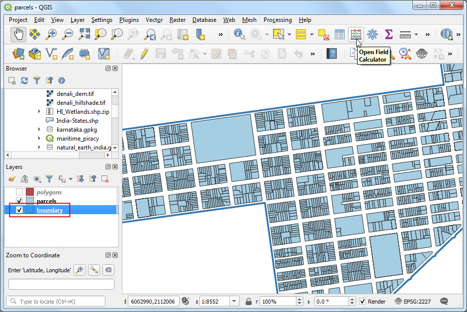
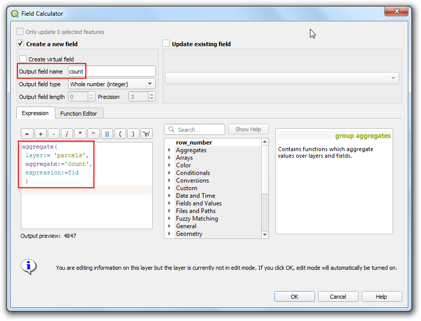
Add a new field named count with the following expression. The expression is reading the features from the parcels layer and giving an aggregate count of the features. You will notice that the the result will be displayed at the bottom of the window.

aggregate(
 layer:= 'parcels',
 aggregate:='count',
 expression:=fid
 )

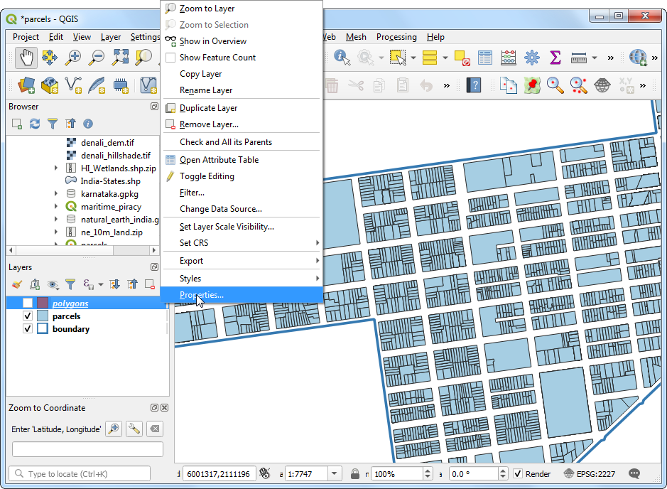
Now we can apply the same concept in a dynamic calculation. Back in the main QGIS window, select the polygons layer and right-click it. Select Properties.

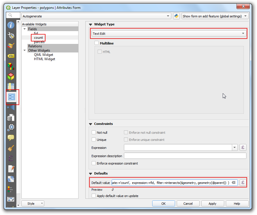
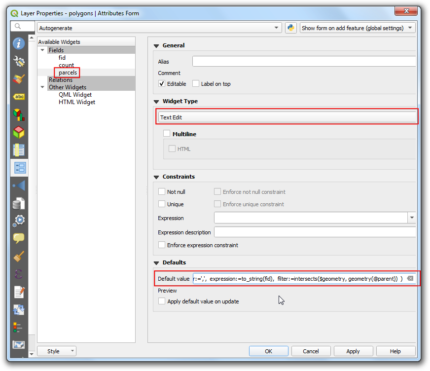
Switch to the Attributes Form tab. Select the field count and choose Text Edit as the Widget Type. At the Default Value field at the bottom, enter the following expression. Note that additional filter value. Here the $geometry refers to the geometry of the parcels layer and geometry(@parent) refers to the geometry of feature from the polygons layer. Click OK.

aggregate(
 layer:= 'parcels',
 aggregate:='count',
 expression:=fid,
 filter:=intersects($geometry, geometry(@parent))
 )

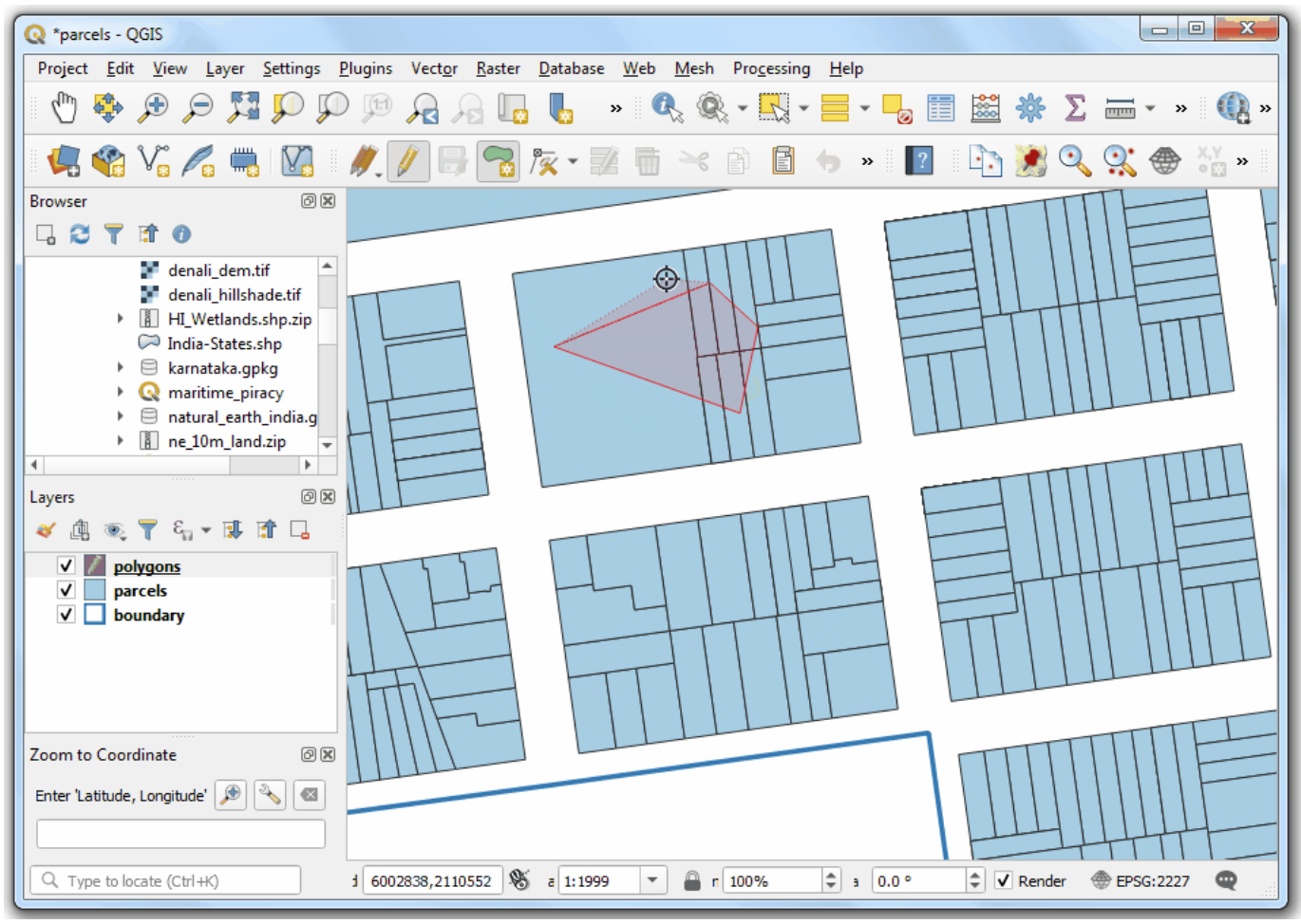
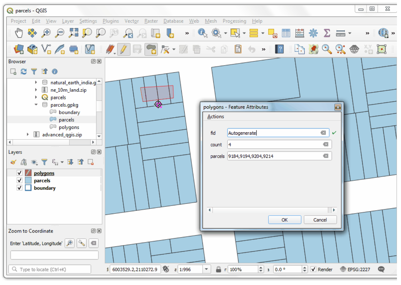
Back in QGIS, click the Toggle Editing button and draw a polygon using the Add Polygon Feature button. Right-click to finish the drawing. As soon as you finish, the count of intersecting features will be calculated by the aggregate expression and displayed in the count field.

View Animated GIF ↗

There are many different types of aggregates available. We can use an aggregate called concatenate to compute a comma-separated text of all feature ids. Go to the Attribute Form properties again and select the parcels field. Enter the following expression as the Default Value.

aggregate(
 layer:= 'parcels',
 aggregate:='concatenate',
 concatenator:=',',
 expression:=to_string(fid),
 filter:=intersects($geometry, geometry(@parent))
 )

Now when to add a new feature, all the intersecting feature ids will be displayed along with the count.

View Animated GIF ↗

Learn more

Apart from aggregate(), there are other advanced functions such as array_foreach() and eval() that are very powerful. Learn about them in the following video where I explain some use cases.

Data Credits

OpenStreetMap (osm) data layers: Data/Maps Copyright 2019 Geofabrik GmbH and OpenStreetMap Contributors. OSM India free extract downloaded from Geofabrik.
India State boundary: Downloaded from Datameet Spatial Data repository.
Anti-shipping Activity Messages: Maritime Safety Information portal , National Geospatial-Intelligence Agency
Land boundaries: Made with Natural Earth. Free vector and raster map data @ naturalearthdata.com.
Road Network: District of Columbia Open Data Catalog.
Alaska IFSAR DTM distributed by USGS Earth Resources Observation and Science (EROS), Downloaded from USGS Earth Explorer
Parcels and Neighborhood boundaries downloaded from DataSF Open Data Portal

授权协议

本课程材料采用知识共享署名-非商业性4.0国际许可协议授权。你可以为任何非商业目的自由使用该材料。请适当注明原作者的名字。

本中文翻译版本禁止商用。

如果你想利用英文原版内容作为商业产品的一部分，需要联系英文原作者询问价格和使用条款，获得培训授权，付对应费用。