今天这段依然出自艾伦·图灵（Alan Turing）1936年发表的经典论文《论可计算数及其在判定问题上的应用》（Alan Turing, On Computable Numbers, with an Application to the Entscheidungsproblem, 1936），具体是文章的第七章。

本章看似繁琐，实则是图灵对通用机器设计的详尽蓝图。他不仅构建了理论上的“硬件”，更开创性地定义了原始指令集与编程语言，并阐明了程序跨机器执行的一致性，是现代计算机体系结构的奠基之作。阅读的时候掌握思路即可，不用沉溺于细节。

原文

7. Detailed description of the universal machine.

A table is given below of the behaviour of this universal machine. The m-configurations of which the machine is capable are all those occurring in the first and last columns of the table, together with all those which occur when we write out the unabbreviated tables of those which appear in the table in the form of m-functions. E.g., e(anf) appears in the table and is an m-function. Its unabbreviated table is (see p. 239)

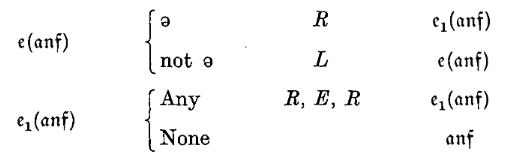
Consequently $e_1(\text{anf})$ is an $m$-configuration of $\mathcal{U}$.

When $\mathcal{U}$ is ready to start work the tape running through it bears on it the symbol $ə$ on an $F$-square and again $ə$ on the next $E$-square; after this, on $F$-squares only, comes the S.D of the machine followed by a double colon "::" (a single symbol, on an $F$-square). The S.D consists of a number of instructions, separated by semi-colons.

Each instruction consists of five consecutive parts

(i) "$D$" followed by a sequence of letters "$A$". This describes the relevant $m$-configuration.

(ii) "$D$" followed by a sequence of letters "$C$". This describes the scanned symbol.

(iii) "$D$" followed by another sequence of letters "$C$". This describes the symbol into which the scanned symbol is to be changed.

(iv) "$L$", "$R$", or "$N$", describing whether the machine is to move to left, right, or not at all.

(v) "$D$" followed by a sequence of letters "$A$". This describes the final $m$-configuration.

The machine $\mathcal{U}$ is to be capable of printing "$A$", "$C$", "$D$", "$0$", "$1$", "$u$", "$v$", "$w$", "$x$", "$y$", "$z$". The S.D is formed from ";", "$A$", "$C$", "$D$", "$L$", "$R$", "$N$".

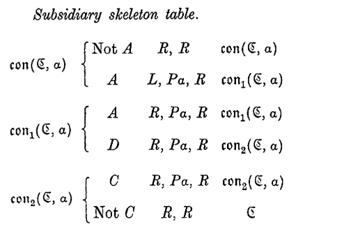
$\text{con}(\mathfrak{C}, \alpha)$. Starting from an $F$-square, $S$ say, the sequence $C$ of symbols describing a configuration closest on the right of $S$ is marked out with letters $\alpha$. $\to \mathfrak{C}$.

$\text{con}(\mathfrak{C}, )$. In the final configuration the machine is scanning the square which is four squares to the right of the last square of $C$. $C$ is left unmarked.

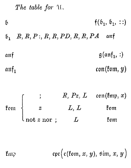
$\mathfrak{b}$. The machine prints $:!:əə0$ on the $F$-squares after $::$. $\to \text{anf}$.

$\text{anf}$. The machine marks the configuration in the last complete configuration with $y$. $\to \text{kom}$.

$\text{kom}$. The machine finds the last semi-colon not marked with $z$. It marks this semi-colon with $z$ and the configuration following it with $x$.

$\text{kmp}$. The machine compares the sequences marked $x$ and $y$. It erases all letters $x$ and $y$. $\to \text{sim}$ if they are alike. Otherwise $\to \text{kom}$.

$\text{anf}$. Taking the long view, the last instruction relevant to the last configuration is found. It can be recognised afterwards as the instruction following the last semi-colon marked $z$. $\to \text{sim}$.

$\text{sim}$. The machine marks out the instructions. That part of the instructions which refers to operations to be carried out is marked with $u$, and the final $m$-configuration with $y$. The letters $z$ are erased.

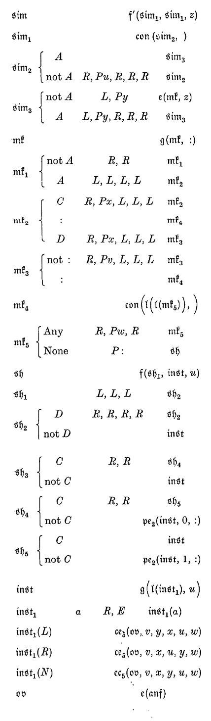
$\text{mk}$. The last complete configuration is marked out into four sections. The configuration is left unmarked. The symbol directly preceding it is marked with $x$. The remainder of the complete configuration is divided into two parts, of which the first is marked with $v$ and the last with $w$. A colon is printed after the whole. $\to \text{sh}$.

$\text{sh}$. The instructions (marked $u$) are examined. If it is found that they involve "Print $0$" or "Print $1$", then $0:$ or $1:$ is printed at the end.

$\text{inst}$. The next complete configuration is written down, carrying out the marked instructions. The letters $u, v, w, x, y$ are erased. $\to \text{anf}$.

翻译

7. 通用机器的详细描述

下表详述了这台通用机器的行为逻辑。该机器所能呈现的 $m$-构型，既涵盖了表中第一列与最后一列明确列出的所有构型，也包含那些以 $m$-函数形式 简写出现的构型——当将其展开为完整的指令表时，其中涉及的所有构型均属此列。例如，$e(\text{anf})$ 这一项作为 $m$-函数出现在表中，其对应的完整指令表如下（参见第 239 页，译者注：对应原文第四章）：

因此，$e_1(\text{anf})$ 也是归属于 $\mathcal{U}$ 的 $m$-构型。

当 $\mathcal{U}$ 准备就绪开始运行时，其纸带的布局如下：首先是一个印有符号 $ə$ 的 $F$-方格，紧随其后的 $E$-方格上也印有 $ə$。在此之后，仅在 $F$-方格上记录机器的标准描述（S.D），并在末尾以双冒号“::”（这是一个占据单个 $F$-方格的特殊符号）作为结束。S.D 由一系列指令构成，指令之间以分号隔开。

每一条指令均由五个连续的部分构成：

(i) “$D$”后紧跟一串字母“$A$”。这部分描述了相关的 $m$-构型。 (ii) “$D$”后紧跟一串字母“$C$”。这部分描述了被扫描的符号。 (iii) “$D$”后紧跟另一串字母“$C$”。这部分描述了扫描符号将被替换成的新符号。 (iv) “$L$”、“$R$”或“$N$”，分别指示机器向左移动、向右移动或保持原地不动。 (v) “$D$”后紧跟一串字母“$A$”。这部分描述了操作完成后的最终 $m$-构型。

通用机器 $\mathcal{U}$ 能够打印的字符集合包括：“$A$”、“$C$”、“$D$”、“$0$”、“$1$”、“$u$”、“$v$”、“$w$”、“$x$”、“$y$”、“$z$”。而 S.D 则是由“;”、“$A$”、“$C$”、“$D$”、“$L$”、“$R$”、“$N$”组合而成的。

$\text{con}(\mathfrak{C}, \alpha)$。从某个 $F$-方格（记为 $S$）起步，向右寻找最近的一个描述构型的符号序列 $C$，并用字母 $\alpha$ 对其进行标记。随后进入状态 $\mathfrak{C}$。

$\text{con}(\mathfrak{C}, )$。在最终的构型中，机器将停留在 $C$ 序列最后一个方格右侧的第四个方格上。此时 $C$ 序列保持未标记状态。

$\mathfrak{b}$。机器在双冒号 $::$ 之后的 $F$-方格区域打印 $:!:əə0$。随后进入状态 $\text{anf}$。

$\text{anf}$。机器在最后一个完整构型中，用 $y$ 标记出其中的“构型”部分。随后进入状态 $\text{kom}$。

$\text{kom}$。机器查找最后一个尚未被 $z$ 标记的分号。它用 $z$ 标记该分号，并用 $x$ 标记紧随该分号之后的“构型”部分。

$\text{kmp}$。机器对比分别被 $x$ 和 $y$ 标记的序列。比对完成后，擦除所有的 $x$ 和 $y$ 标记。若两序列相同，则进入状态 $\text{sim}$；否则，返回状态 $\text{kom}$。

$\text{anf}$（注：这是对上述过程的总结）。从宏观视角来看，这一步旨在为当前的构型找到相关的最后一条指令。该指令在后续可以通过识别它紧跟在最后一个被标记为 $z$ 的分号之后而被确认。随后进入状态 $\text{sim}$。

$\text{sim}$。机器对指令进行标记：将指令中涉及具体操作的部分标记为 $u$，将最终的 $m$-构型部分标记为 $y$。同时，擦除字母 $z$。

$\text{mk}$。将最后一个完整构型划分为四个区块：其“构型”部分保持不标记；紧邻其左侧的符号标记为 $x$；完整构型的剩余部分分为两段，第一段标记为 $v$，最后一段标记为 $w$。最后，在整个序列的末尾打印一个冒号。随后进入状态 $\text{sh}$。

$\text{sh}$。检查被 $u$ 标记的指令内容。若发现指令中包含“打印 $0$”或“打印 $1$”的操作，则相应地在序列末尾打印 $0:$ 或 $1:$。

$\text{inst}$。执行被标记的指令，写下新的完整构型。随后擦除字母 $u, v, w, x, y$。最后返回状态 $\text{anf}$。

逐段解析

1. 通用图灵机 $\mathcal{U}$ 的初始化

“当 $\mathcal{U}$ 准备开始工作时，穿过它的纸带... 是机器的 S.D，后面跟一个双冒号 :: ...”

• 输入格式：$\mathcal{U}$ 的纸带布局经过精心设计。
• 程序区：开头记录的是 S.D（源代码），例如 DADDCRDAA;DAADDRDAAA;...。
• 分隔符：使用 :: 将“程序”与“运行数据”隔开。
• 数据区：在 :: 之后，$\mathcal{U}$ 将记录目标机器 $\mathcal{M}$ 的运行状态。初始状态通常写作 :: ə ə 0（即 $\mathcal{M}$ 的初始快照）。

2. 指令解析循环（The Fetch-Execute Cycle）

$\mathcal{U}$ 的运行过程是一个无限循环，完美对应了现代 CPU 的 取指-解码-执行（Fetch-Decode-Execute）周期。

1. 定位当前状态 ($\text{anf}$)：

   • $\mathcal{U}$ 首先需要读取数据区中 $\mathcal{M}$ 的当前状态（即最后一个完整构型）。
   • 它使用标记 $y$ 标出 $\mathcal{M}$ 当前的内部状态和正在扫描的符号。

2. 查找匹配指令 ($\text{kom}, \text{kmp}$)：

   • $\mathcal{U}$ 返回程序区（S.D），逐条扫描指令。
   • 每条指令都包含一个“触发条件”（特定状态 + 特定符号）。
   • $\mathcal{U}$ 将指令的触发条件（标记为 $x$）与 $\mathcal{M}$ 的当前状态（标记为 $y$）进行比较。
   • 如果匹配，则进入下一步；如果不匹配，则继续寻找下一条指令。

3. 执行指令 ($\text{sim}, \text{mk}, \text{inst}$)：

   • 一旦找到匹配指令，$\mathcal{U}$ 便读取指令的后半部分（执行动作 + 新状态）。
   • 打印/移动：$\mathcal{U}$ 在数据区末尾写下新的完整构型，相当于生成了 $\mathcal{M}$ 下一时刻的快照。
   • 清理：擦除辅助标记 $x, y, z$ 等，为下一轮循环做准备。

3. 辅助标记的作用

“机器 $\mathcal{U}$ 能够打印... $u, v, w, x, y, z$...”

• 元变量：这些字母（$u, v, x, y, z$ 等）从未出现在 $\mathcal{M}$ 的原始纸带上，它们是 $\mathcal{U}$ 专用的指针或高亮标记。
• 标记法 (Marking)：由于图灵机无法像高级语言（如 C 语言）那样定义变量或指针，它只能通过在目标符号旁边的 $E$-方格内写入特殊字符（如 $x$）来表示“当前关注的是这个符号”。
• 比较逻辑：$\text{kmp}$ 状态生动展示了图灵机如何比较两个字符串是否相等——它必须在两个字符串之间来回移动，逐个比对被标记的字符。

总结

这一章是整篇论文在工程实现上的高潮。图灵手把手地演示了如何用一台图灵机去模拟另一台图灵机。 1. 解释器的原型：$\mathcal{U}$ 的逻辑结构可以看作是对应了现代编程语言解释器（如 Python 解释器）的主循环机制。 2. 复杂性的物理基础：虽然原理看似简单，但实现细节（如查找、匹配、复制、移动）极其繁琐。这解释了为何现代 CPU 需要数十亿个晶体管——正是为了在硬件层面高效地处理这些基本操作。 3. 完备性证明：通过详细构造出 $\mathcal{U}$，图灵证明了“通用计算”不仅是数学上的理论存在，更是物理上可实现的工程现实。